Neural Network Architectures for EEG-Decoding

Three progressively more generic architectures

• Shallow ConvNet learns temporal filters and later average-pools over large timeregions

• Deep ConvNet uses smaller temporal filters and max-pooling over small timeregions

• Residual network uses many layers with even smaller temporal filters

We continued developing our neural network architectures with our EEG-specific development strategy of starting with networks that resemble feature-based algorithms. After the filterbank network from the master thesis, we adapted the so-called shallow ConvNet, initally also developed in the same master thesis [Schirrmeister, 2015]. The shallow ConvNet still resembles filter bank common spatial patterns, but less closely than the filterbank network. After validating that these initial network architectures perform as well as filter bank common spatial patterns, we progressed to developing and evaluating more generic architectures, namely the deep ConvNet and the residual ConvNet.

In this section, I describe the architectures presented in our first publication on EEG deep learning decoding [Schirrmeister et al., 2017]. This part uses text and figures from [Schirrmeister et al., 2017] adapted for readibility in this thesis. The deep and residual ConvNet were primarily developed by me together with help from my coauthors.

Shallow ConvNet Architecture

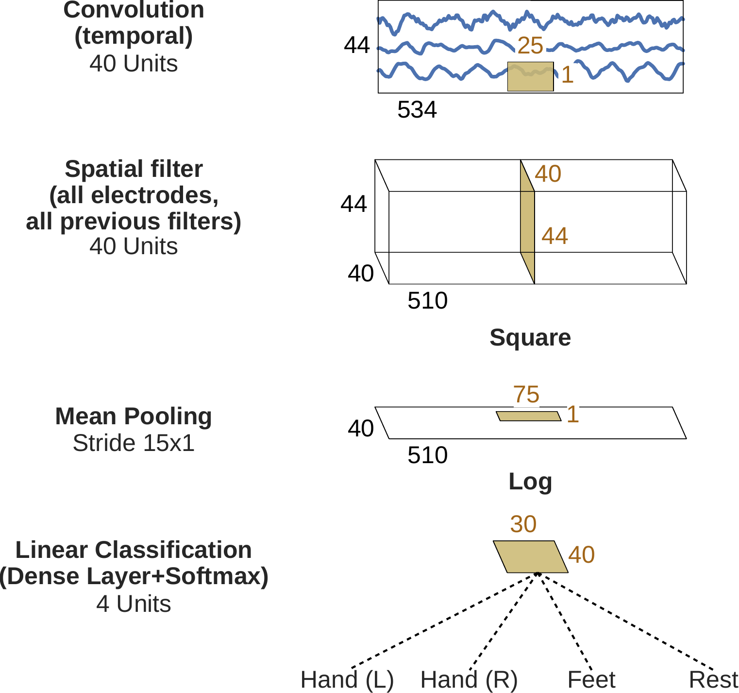
Fig. 5 Shallow ConvNet architectur EEG input (at the top) is progressively transformed toward the bottom, until the final classifier output. Black cuboids: inputs/feature maps; brown cuboids: convolution/pooling kernels. The corresponding sizes are indicated in black and brown, respectively. Note that the final dense layer operates only on a small remaining temporal dimension, making it similar to a regular convolutional layer. Figure from [Schirrmeister et al., 2017].

We developed the shallow ConvNet architecture, a more flexible architecture than the filterbank network that also learns temporal filters on the input signal and on the later representation. Instead of bandpass-filtered signals, it is fed the raw signals as input. The steps the architecture implements are as follows (also see Fig. 5):

1. Temporal Filtering Learnable temporal filters are indepedently convolved with the signals of each EEG electrode. Afterwards, the channel dimension of the network representation contains \(\mathrm{electrodes} \cdot \mathrm{temporal~ filters}\) channels.

2. Spatial Filtering Combining spatial filtering with mixing the outputs of the temporal filters, the network-channel dimension is linearly transformed by learned weights to a smaller dimensionality for further preprocessing.

3. Log Average Power The resulting feature timeseries are then squared, average-pooled and log-transformed, which allows the network to more easily learn log-power-based features. Unlike the filterbank network, the average pooling does not collapse the feature timeseries into one value per trial. So after these processing steps, still some temporal information about the timecourse of the variance throughout the trial can be preserved.

4. Classifier The final classification layer transforms these feature timecourses into class probabilities using a linear transformation and a softmax function.

Deep ConvNet Architecture

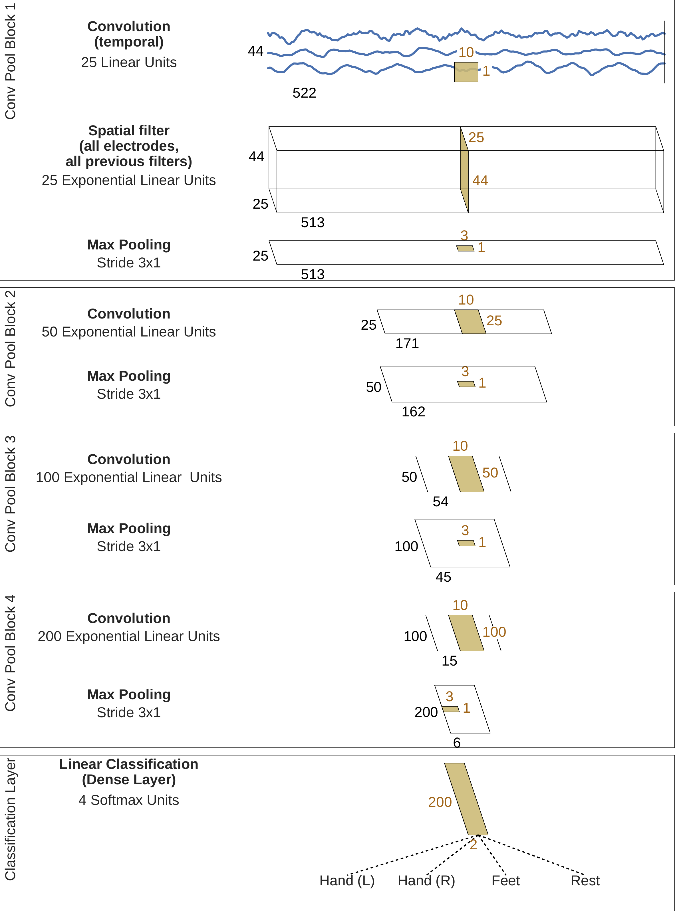
Fig. 6 Deep ConvNet architecture.. Conventions as in Fig. 5. Figure from [Schirrmeister et al., 2017]

The deep ConvNet is a more generic architecture, closer to network architectures used in computer vision, see Fig. 6 for a schematic overview. The first two temporal convolution and spatial filtering layers are the same in the shallow network, which is followed by a ELU nonlinearity (ELUs, \(f(x)=x\) for \(x > 0\) and \(f(x) = e^x-1\) for \(x <= 0\) [Clevert et al., 2016]) and max pooling. The following three blocks simply consist of a convolution, a ELU nonlinearity and a max pooling. In the end, there is again a final linear classification layer with a softmax function. Due to its less specific and more generic computational steps, the deep architecture should be able to capture a large variety of features. Hence, the learned features may also be less biased towards the amplitude features commonly used in task-related EEG decoding.

Residual ConvNet Architecture

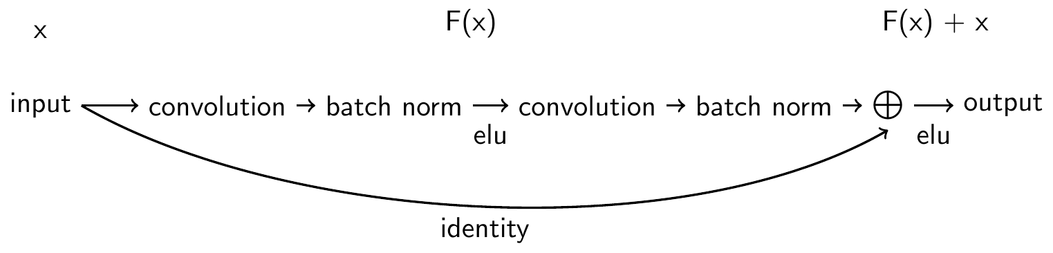
Fig. 7 Residual block. Residual block used in the ResNet architecture and as described in original paper ([He et al., 2015]; see Fig. 2) with identity shortcut option A, except using ELU instead of ReLU nonlinearities. Figure from [Schirrmeister et al., 2017]

Table 4 Residual ConvNet architecture hyperparameters. Number of kernels, kernel and output size for all subparts of the network. Output size is always time x height x channels. Note that channels here refers to input channels of a network layer, not to EEG channels; EEG channels are in the height dimension. Output size is only shown if it changes from the previous block. Second convolution and all residual blocks used ELU nonlinearities. Note that in the end we had seven outputs, i.e., predictions for the four classes, in the time dimension (7x1x4 final output size). In practice, when using cropped training as explained in the following chapter, we even had 424 predictions, and used the mean of these to predict the trial.

Layer/Block	Number of Kernels	Kernel Size	Output Size
Input			1000x44x1
Convolution (linear)	48	3x1	1000x44x48
Convolution (ELU)	48	1x44	1000x1x48
ResBlock (ELU)	48	3x1
ResBlock (ELU)	48	3x1
ResBlock (ELU)	96	3x1 (Stride 2x1)	500x1x96
ResBlock (ELU)	96	3x1
ResBlock (ELU)	144	3x1 (Stride 2x1)	250x1x96
ResBlock (ELU)	144	3x1
ResBlock (ELU)	144	3x1 (Stride 2x1)	125x1x96
ResBlock (ELU)	144	3x1
ResBlock (ELU)	144	3x1 (Stride 2x1)	63x1x96
ResBlock (ELU)	144	3x1
ResBlock (ELU)	144	3x1 (Stride 2x1)	32x1x96
ResBlock (ELU)	144	3x1
ResBlock (ELU)	144	3x1 (Stride 2x1)	16x1x96
ResBlock (ELU)	144	3x1
Mean Pooling		10x1	7x1x144
Convolution + Softmax	4	1x1	7x1x4

We also developed a residual ConvNet ([He et al., 2015]) for EEG decoding. Residual networks add the input of a residual computational block back to its output, and this allows to stably train much deeper networks. We use the same residual blocks as the original paper, described in Figure Fig. 7. Our residual ConvNet used ELU activation functions throughout the network (same as the deep ConvNet) and also starts with a splitted temporal and spatial convolution (same as the deep and shallow ConvNets), followed by 14 residual blocks, mean pooling and a final softmax dense classification layer.

In total, the residual ConvNet has 31 convolutional layers, a depth where ConvNets without residual blocks started to show problems converging in the original residual networks paper [He et al., 2015]. In layers where the number of channels is increased, we padded the incoming feature map with zeros to match the new channel dimensionality for the shortcut, as in option A of the original paper [He et al., 2015]. The overall architecture is also shown in Table 4.

Open Questions

• How do these three architectures compare against each other on movement-related decoding tasks?