Decoding Movement-Related Brain Activity#
ConvNets can perform as well as FBCSP on movement-related decoding
Shallow network performs best on highpassed data
Deep network strongly benefits from cropped training on non-highpassed data
Residual network performs well with right initialization
Methodological improvements from computer vision improve EEG deep learning decoding
Visualizations reveal use of spectral power features with neurophysiologically plausible patterns
Movement-related decoding problems are among the most researched in EEG decoding and were hence our problem of choice for the first evaluation of deep learning on EEG. A typical movement-related experimental setting is that subjects receive a cue for a specific body part (e.g. right hand, feet, tongue, etc.) and either move (motor execution) or imagine to move (motor imagery) this body part. The EEG signals recorded during the imagined or executed movements then often contain patterns specific to the body part being moved or thought about. These patterns can then be decoded using machine learning. In the following, I will describe our study on movement-related EEG decoding using deep learning, mostly using content adapted from Schirrmeister et al. [2017] and from [Hartmann et al., 2018]. The main study as published in Schirrmeister et al. [2017] was carried out by me as the main author with help of al the coauthors. For Hartmann et al. [2018], Kay Hartmann was the main contributor and I supported and advised him.
Datasets#
High-Gamma Dataset#
Our High-Gamma Dataset is a 128-electrode dataset (of which we later only use 44 sensors covering the motor cortex) obtained from 14 healthy subjects (6 female, 2 left-handed, age 27.2\(\pm\)3.6 (mean\(\pm\)std)) with roughly 1000 (963.1\(\pm\)150.9, mean\(\pm\)std) four-second trials of executed movements divided into 13 runs per subject. The four classes of movements were movements of either the left hand, the right hand, both feet, and rest (no movement, but same type of visual cue as for the other classes). The training set consists of the approx. 880 trials of all runs except the last two runs, the test set of the approx. 160 trials of the last 2 runs. This dataset was acquired in an EEG lab optimized for non-invasive detection of high-frequency movement-related EEG components [Ball et al., 2008, Darvas et al., 2010]. Such high-frequency components in the range of approx. 60 to above 100 Hz are typically increased during movement execution and may contain useful movement-related information [Crone et al., 1998, Hammer et al., 2016, Quandt et al., 2012]. Our technical EEG Setup comprised (1.) Active electromagnetic shielding: optimized for frequencies from DC - 10 kHz (-30 dB to -50 dB), shielded window, ventilation & cable feedthrough (mrShield, CFW EMV-Consulting AG, Reute, CH) (2.) Suitable amplifiers: high-resolution (24 bits/sample) and low-noise (\textless{}0.6 \(\mu V\) RMS 0.16–200 Hz, 1.5 \(\mu V\) RMS 0.16–3500 Hz), 5 kHz sampling rate (NeurOne, Mega Electronics Ltd, Kuopio, FI) (3.) actively shielded EEG caps: 128 channels (WaveGuard Original, ANT, Enschede, NL) and (4.) full optical decoupling: All devices are battery powered and communicate via optic fibers.
Subjects sat in a comfortable armchair in the dimly lit Faraday cabin. The contact impedance from electrodes to skin was typically reduced below 5 kOhm using electrolyte gel (SUPER-VISC, EASYCAP GmbH, Herrsching, GER) and blunt cannulas. Visual cues were presented using a monitor outside the cabin, visible through the shielded window. The distance between the display and the subjects’ eyes was approx. 1 m. A fixation point was attached at the center of the screen. The subjects were instructed to relax, fixate the fixation mark and to keep as still as possible during the motor execution task. Blinking and swallowing was restricted to the inter-trial intervals. The electromagnetic shielding combined with the comfortable armchair, dimly lit Faraday cabin and the relatively long 3-4 second inter-trial intervals (see below) were used to minimize artifacts produced by the subjects during the trials.
The tasks were as following. Depending on the direction of a gray arrow that was shown on black background, the subjects had to repetitively clench their toes (downward arrow), perform sequential finger-tapping of their left (leftward arrow) or right (rightward arrow) hand, or relax (upward arrow). The movements were selected to require little proximal muscular activity while still being complex enough to keep subjects involved. Within the 4-s trials, the subjects performed the repetitive movements at their own pace, which had to be maintained as long as the arrow was showing. Per run, 80 arrows were displayed for 4 s each, with 3 to 4 s of continuous random inter-trial interval. The order of presentation was pseudo-randomized, with all four arrows being shown every four trials. Ideally 13 runs were performed to collect 260 trials of each movement and rest. The stimuli were presented and the data recorded with BCI2000 [Schalk et al., 2004]. The experiment was approved by the ethical committee of the University of Freiburg.
BCI Competition IV 2a#
The BCI competition IV dataset 2a is a 22-electrode EEG motor-imagery dataset, with 9 subjects and 2 sessions, each with 288 four-second trials of imagined movements per subject (movements of the left hand, the right hand, the feet and the tongue), for details see Brunner et al. [2008]. The training set consists of the 288 trials of the first session, the test set of the 288 trials of the second session.
BCI Competition IV 2b#
The BCI competition IV dataset 2b is a 3-electrode EEG motor-imagery dataset with 9 subjects and 5 sessions of imagined movements of the left or the right hand, the latest 3 sessions include online feedback [Leeb et al., 2008]. The training set consists of the approx. 400 trials of the first 3 sessions (408.9\(\pm\)13.7, mean\(\pm\)std), the test set consists of the approx. 320 trials (315.6\(\pm\)12.6, mean\(\pm\)std) of the last two sessions.
Preprocessing#
We only minimally preprocessed the data to allow the networks to extract as much information as possible while keeping the input distribution in a value range suitable for stable network training.
Concretely, our preprocessing steps were:
Remove outlier trials: Any trial where at least one channel had a value outside +- 800 mV was removed to ensure stable training.
Channel selection: For the high-gamma dataset, we selected only the 44 sensors covering the motor cortex for faster and more accurate motor decoding.
High/bandpass (Optional) : Highpass signal to above 4 Hz. This should partially remove potentially informative eye components from the signal and ensure that the decoding relies more on brain signals. For the BCI competition datasets, in this step we bandpassed to 4-38 Hz as using only frequencies until ~38-40 Hz was commonly done in prior work in this dataset.
Standardization: Exponential moving standardization as described below to make sure the input distribution value range is suitable for network training.
Our electrode-wise exponential moving standardization computes exponential moving means and variances with a decay factor of 0.999 for each channel and used these to standardize the continuous data. Formally,
\(\mu_t = 0.001 x_t + 0.999\mu_{t-1}\)
\(\sigma_t^2 = 0.001(x_t - \mu_t)^2 + 0.999 \sigma_{t-1}^2\)
\(x't = (x_t - \mu_t) / \sqrt{\sigma_t^2}\)
where \(x't\) and \(x_t\) are the standardized and the original signal for one electrode at time \(t\), respectively. As starting values for these recursive formulas we set the first 1000 mean values \(\mu_t\) and first 1000 variance values \(\sigma_t^2\) to the mean and the variance of the first 1000 samples, which were always completely inside the training set (so we never used future test data in our preprocessing). Some form of standardization is a commonly used procedure for ConvNets; exponentially moving standardization has the advantage that it is also applicable for an online BCI.
For FBCSP, this standardization always worsened accuracies in preliminary experiments, so we did not use it. Overall, the minimal preprocessing without any manual feature extraction ensured our end-to-end pipeline could in principle be applied to a large number of brain-signal decoding tasks as we validated later, see Generalization to Other Tasks.
Training Details#
As our optimization method, we used Adam [Kingma and Ba, 2014] together with a specific early stopping method, as this consistently yielded good accuracy in preliminary experiments on the training set. Adam is a variant of stochastic gradient descent designed to work well with high-dimensional parameters, which makes it suitable for optimizing the large number of parameters of a ConvNet [Kingma and Ba, 2014]. The early stopping strategy that we use throughout these experiments, developed in the computer vision field 1, splits the training set into a training and validation fold and stops the first phase of the training when validation accuracy does not improve for a predefined number of epochs. The training continues on the combined training and validation fold starting from the parameter values that led to the best accuracies on the validation fold so far. The training ends when the loss function on the validation fold drops to the same value as the loss function on the training fold at the end of the first training phase (we do not continue training in a third phase as in the original description). Early stopping in general allows training on different types of networks and datasets without choosing the number of training epochs by hand. Our specific strategy uses the entire training data while only training once. In our study, all reported accuracies have been determined on an independent test set.
Note that in later works we do not use this early stopping method anymore as we found training on the whole training set with a cosine learning rate schedule [Loshchilov and Hutter, 2017] to lead to better final decoding performance.
Design Choices#
Design aspect |
Our Choice |
Variants |
Motivation |
|---|---|---|---|
Activation functions |
ELU |
Square, ReLU |
We expected these choices to be sensitive to the type of feature (e.g., signal phase or power), as squaring and mean pooling results in mean power (given a zero-mean signal). Different features may play different roles in the low-frequency components vs the higher frequencies (see the section “Datasets and Preprocessing”). |
Pooling mode |
Max |
Mean |
(see above) |
Regularization and intermediate normalization |
Dropout + batch normalization + a new tied loss function (explanations see text) |
Only batch normalization, only dropout, neither of both, nor tied loss |
We wanted to investigate whether recent deep learning advances improve accuracies and check how much regularization is required. |
Factorized temporal convolutions |
One 10 × 1 convolution per convolutional layer |
Two 6 × 1 convolutions per convolutional layer |
Factorized convolutions are used by other successful ConvNets [Szegedy et al., 2015] |
Splitted vs one-step convolution |
Splitted convolution in first layer (see the section “Deep ConvNet for raw EEG signals”) |
One-step convolution in first layer |
Factorizing convolution into spatial and temporal parts may improve accuracies for the large number of EEG input channels (compared with three rgb color channels of regular image datasets). |
For the shallow and deep network, we evaluated how a number of design choices affect the final accuracies.
Tied Loss Function#
Our tied loss function penalizes the discrepancy between neighbouring predictions. Concretely, in this tied sample loss function, we added the cross-entropy of two neighboring predictions to the usual loss of of negative log likelihood of the labels. So, denoting the predicted probabilties \(p\big(l_k|f_k(X^j_{t..t+T'};\theta)\big)\) for crop \(X^j_{t..t+T'}\) with label \(l_k\) from time step \(t\) to \(t+T'\) by \(p_{f,k}(X^j_{t..t+T'})\), the loss now also depends on the predicted probabilties for the next crop \(p_{f,k}(X^j_{t..t+T'+1})\) and is then:
\(\textrm{loss}\big(y^j, p_{f,k}(X^j_{t..t+T'})\big)=\sum_{k=1}^{K}-log\big(p_{f,k}(X^j_{t..t+T'})\big)\cdot \delta(y^j=l_k) \quad + \quad \sum_{k=1}^{K}-log\big(p_{f,k}(X^j_{t..t+T'})\big) \cdot p_{f,k}(X^j_{t..t+T'+1})\)
This is meant to make the ConvNet focus on features which are stable for several neighboring input crops.
Results#
Validation of FBCSP Pipeline#
As a first step before moving to the evaluation of ConvNet decoding, we validated our FBCSP implementation, as this was the baseline we compared the ConvNets results against. To validate our FBCSP implementation, we compared its accuracies to those published in the literature for the BCI competition IV dataset 2a [Sakhavi et al., 2015]. Using the same 0.5–2.5 s (relative to trial onset) time window, we reached an accuracy of 67.6%, statistically not significantly different from theirs (67.0%, p=0.73, Wilcoxon signed-rank test). Note however, that we used the full trial window for later experiments comparing against convolutional networks, i.e., from 0.5–4 seconds. This yielded a slightly better accuracy of 67.8%, which was still not statistically significantly different from the original results on the 0.5–2.5 s window (p=0.73). For all later comparisons, we use the 0.5–4 seconds time window on all datasets.
Filterbank Network#
Decoding Method |
Sampling rate |
Test Accuracy [%] |
Std [%] |
|---|---|---|---|
FBCSP |
300 |
88.1 |
13.9 |
FBCSP |
150 |
86.7 |
14.3 |
Filterbank Net |
300 |
90.5 |
10.4 |
Filterbank Net |
150 |
87.9 |
13.9 |
Prior to our more extensive study, we had evaluated the filterbank network on a different version of the High-Gamma Dataset in a master thesis [Schirrmeister, 2015]. This version of the dataset included different subjects, as some subjects had not been recorded yet and other subjects were later excluded for the work here due to the presence of too many artifacts. Furthermore, we evaluated 150Hz and 300 Hz as sampling rates here, in the remainder we will use 250 Hz.
The results in Table 6 show that the Filterbank net outperformed FBCSP by 2.4% (300 Hz) and 1.3% (150 Hz) respectively. Despite the good performance, we did not evaluate this network further after the master thesis due to the very large GPU memory requirement of our implementation and our interest in evaluating more expressive architectures not as tightly constrained to implement FBCSP steps.
ConvNets Reached FBCSP Accuracies#
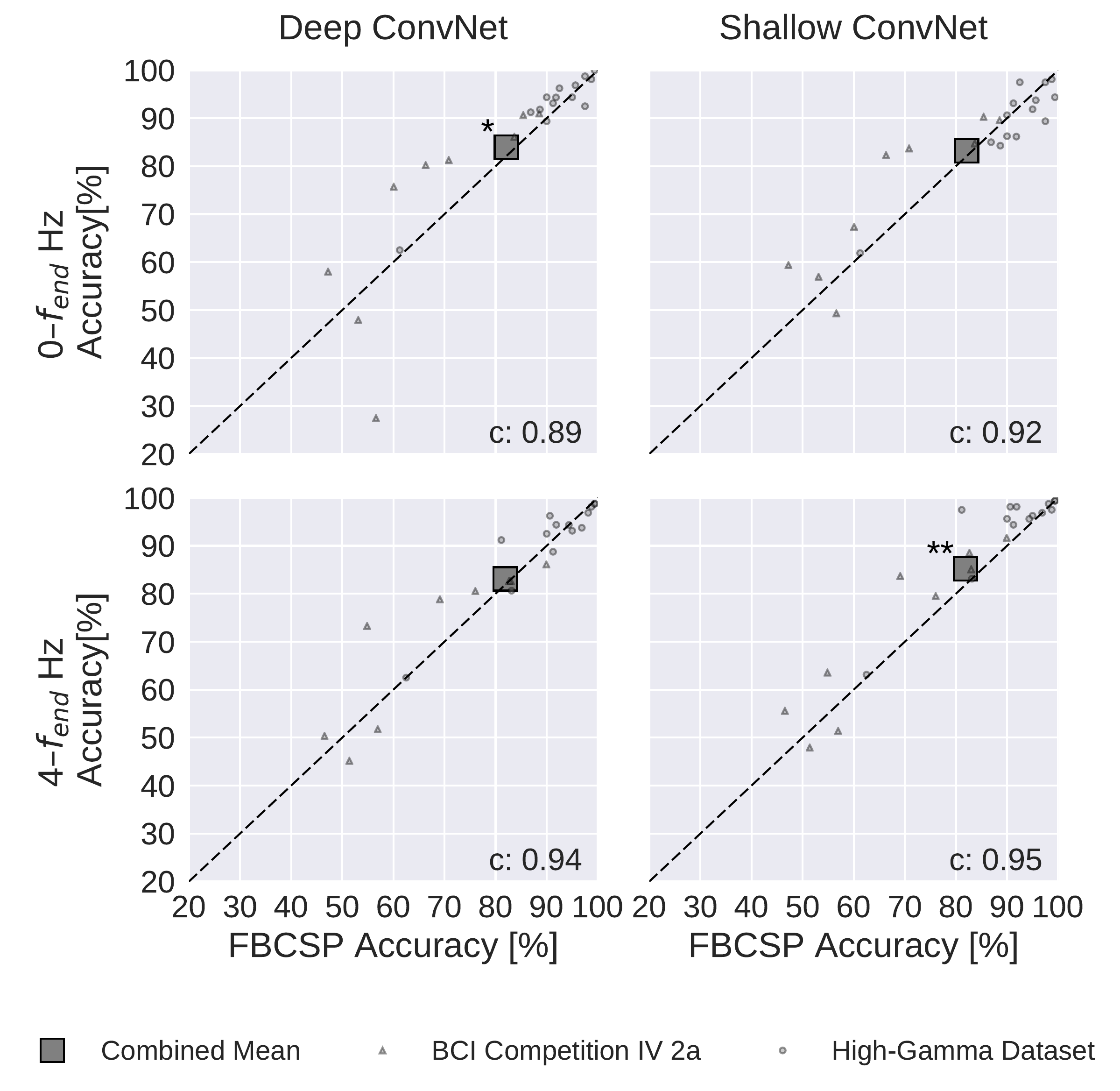
Fig. 20 FBCSP vs. ConvNet decoding accuracies. Each small marker represents accuracy of one subject, the large square markers represent average accuracies across all subjects of both datasets. Markers above the dashed line indicate experiments where ConvNets performed better than FBCSP and opposite for markers below the dashed line. Stars indicate statistically significant differences between FBCSP and ConvNets (Wilcoxon signed-rank test, p<0.05: *, p<0.01: **, p<0.001=***). Bottom left of every plot: linear correlation coefficient between FBCSP and ConvNet decoding accuracies. Mean accuracies were very similar for ConvNets and FBCSP, the (small) statistically significant differences were in direction of the ConvNets. Figure from Schirrmeister et al. [2017].#
Dataset |
Frequency Range (Hz) |
FBCSP |
Deep |
Shallow |
|---|---|---|---|---|
BCIC IV 2a |
0–38 |
68.0 |
+2.9 |
+5.7* |
BCIC IV 2a |
4–38 |
67.8 |
+2.3 |
+4.1 |
HGD |
0–125 |
91.2 |
+1.3 |
-1.9 |
HGD |
4–125 |
90.9 |
+0.5 |
+3.0* |
Combined |
0–\(f_{end}\) |
82.1 |
+1.9* |
+1.1 |
Combined |
4–\(f_{end}\) |
81.9 |
+1.2 |
+3.4** |
Both the deep and the shallow ConvNets, with appropriate design choices (see Design Choices Affected Decoding Performance), reached similar accuracies as FBCSP-based decoding, with small but statistically significant advantages for the ConvNets in some settings. For the mean of all subjects of both datasets, accuracies of the shallow ConvNet on \(0-f_\textrm{end}\) Hz and for the deep ConvNet on \(4-f_\textrm{end}\) Hz were not statistically significantly different from FBCSP (see Fig. 20). The deep ConvNet on \(0-f_\textrm{end}\) Hz and the shallow ConvNet on \(4-f_\textrm{end}\) Hz reached slightly higher (1.9% and 3.3% higher, respectively) accuracies that were also statistically significantly different (P < 0.05, Wilcoxon signed-rank test). Note that all results in this section were obtained with cropped training. Note that all P values below 0.01 in this study remain significant when controlled with false-discovery-rate correction at \(\alpha=0.05\) across all tests involving ConvNet accuracies.
Confusion Matrices are Similar between FBCSP and ConvNets#
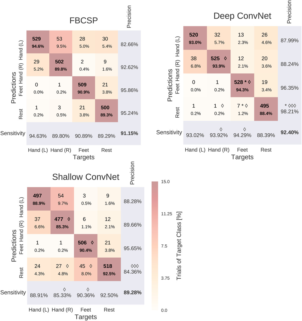
Fig. 21 Confusion matrices for FBCSP- and ConvNet-based decoding. Results are shown for the High-Gamma Dataset, on \(0–f_\textrm{end}\) Hz. Each entry of row r and column c for upper-left 4×4-square: Number of trials of target r predicted as class c (also written in percent of all trials). Bold diagonal corresponds to correctly predicted trials of the different classes. Percentages and colors indicate fraction of trials in this cell from all trials of the corresponding column (i.e., from all trials of the corresponding target class). The lower-right value corresponds to overall accuracy. Bottom row corresponds to sensitivity defined as the number of trials correctly predicted for class c/number of trials for class c. Rightmost column corresponds to precision defined as the number of trials correctly predicted for class r/number of trials predicted as class r. Stars indicate statistically significantly different values of ConvNet decoding from FBCSP, diamonds indicate statistically significantly different values between the shallow and deep ConvNets. P<0.05: \(\diamond\)/*, P<0.01: \(\diamond\diamond\)/**, P<0.001: \(\diamond\diamond\diamond\)/***, Wilcoxon signed-rank test. Figure from Schirrmeister et al. [2017].#
Hand (L) / Hand (R) |
Hand (L) / Feet |
Hand (L) / Rest |
Hand (R) / Feet |
Hand (R) / Rest |
Feet / Rest |
|
|---|---|---|---|---|---|---|
FBCSP |
82 |
28 |
31 |
3 |
12 |
42 |
Deep |
70 |
13 |
27 |
13 |
21 |
26 |
Shallow |
99 |
3 |
34 |
5 |
37 |
73 |
Confusion matrices for the High-Gamma Dataset on 0–\(f_{end}\) Hz were very similar for FBCSP and both ConvNets (see Fig. 21). The majority of all mistakes were due to discriminating between Hand (L) / Hand (R) and Feet / Rest, see Table Table 8. Seven entries of the confusion matrix had a statistically significant difference (p<0.05, Wilcoxon signed-rank test) between the deep and the shallow ConvNet, in all of them the deep ConvNet performed better. Only two differences between the deep ConvNet and FBCSP were statistically significant (p<0.05), none for the shallow ConvNet and FBCSP. Confusion matrices for the BCI competition IV dataset 2a showed a larger variability and hence a less consistent pattern, possibly because of the much smaller number of trials.
Residual ConvNets Can Be Competitive with Improved Training#
Dataset |
Frequency Range (Hz) |
FBCSP |
ResNet Before |
ResNet Now |
|---|---|---|---|---|
BCIC IV 2a |
68.0 |
-0.3 |
+3.7 |
|
BCIC IV 2a |
67.8 |
-7.0* |
-0.9 |
|
HGD |
0–125 |
91.2 |
-2.3* |
+1.1 |
HGD |
4–125 |
90.9 |
-1.1 |
0.0 |
Combined |
0–\(f_{end}\) |
82.1 |
-1.1 |
+2.2 |
Combined |
4–\(f_{end}\) |
81.9 |
-3.5* |
-0.4 |
In our original study, residual ConvNets had underperformed our FBCSP baseline, in several settings even with statistical significance. However, later investigations revealed that better weight initializations, concretely scaling down the weight initialization more strongly, can lead to improved results. In work done for this thesis, I repeated the original experiments using our current decoding pipeline with the residual ConvNets. Table 9 reports the original accuracies and the accuracies obtained with our current codebase. Notably, residual ConvNets no longer substantially underperform FBCSP, even slightly outperforming it in the setting without highpass.
Design Choices Affected Decoding Performance#
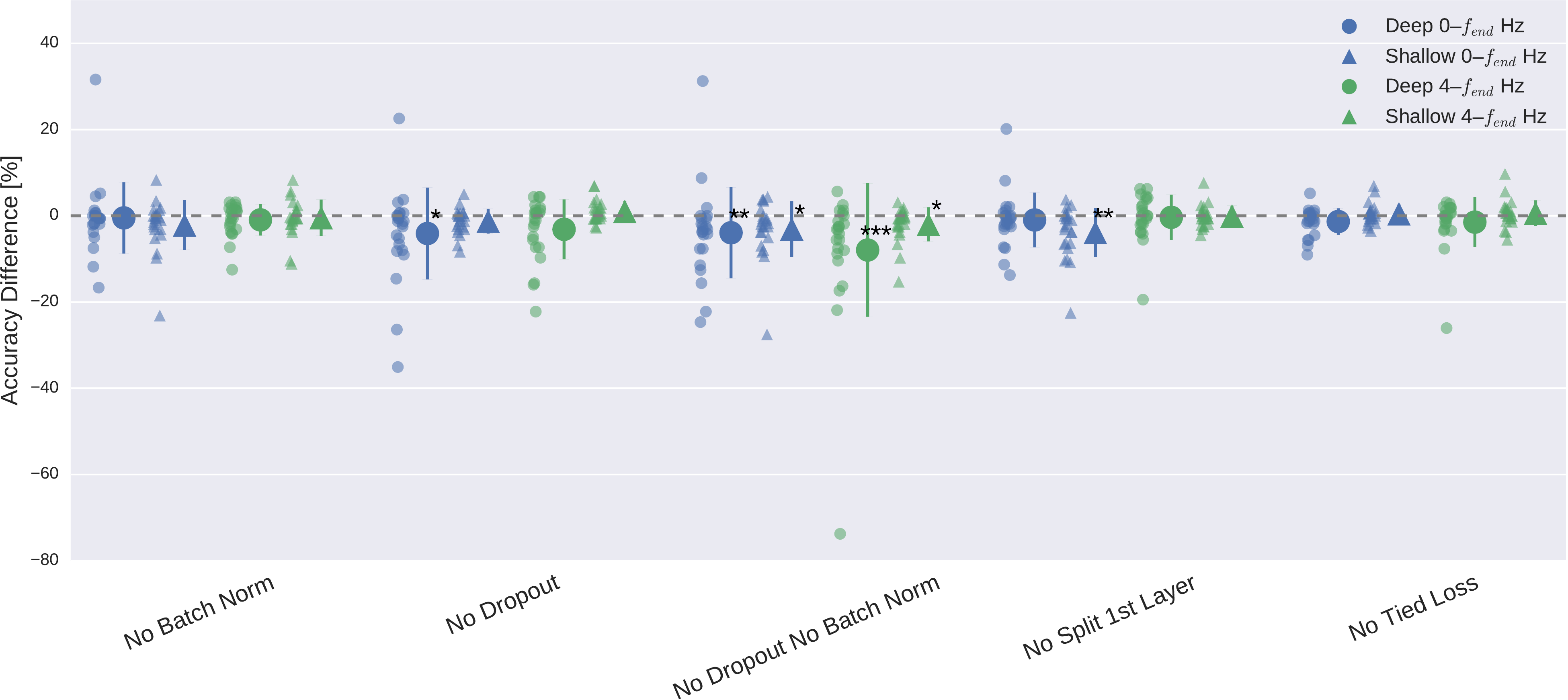
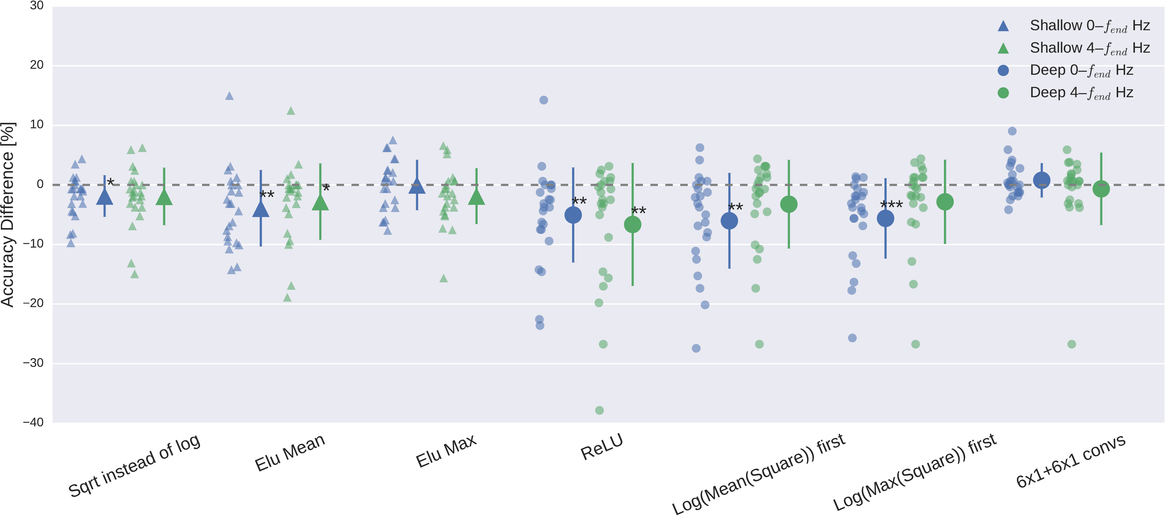
Fig. 22 Impact of ConvNet design choices on decoding accuracy. Accuracy differences of baseline and design choices on x-axis for the \(0-f_\textrm{end}\) Hz and \(4-f_\textrm{end}\) Hz datasets. Each small marker represents accuracy difference for one subject, and each larger marker represents mean accuracy difference across all subjects of both datasets. Bars: standard error of the differences across subjects. Stars indicate statistically significant differences to baseline (Wilcoxon signed-rank test, P < 0.05: \(\diamond\)*, P < 0.01: \(\diamond\diamond\)**, P < 0.001=***). Top: Impact of design choices applicable to both ConvNets. Shown are the effects from the removal of one aspect from the architecture on decoding accuracies. All statistically significant differences were accuracy decreases. Notably, there was a clear negative effect of removing both dropout and batch normalization, seen in both ConvNets’ accuracies and for both frequency ranges. Bottom: Impact of different types of nonlinearities, pooling modes and filter sizes. Results are given independently for the deep ConvNet and the shallow ConvNet. As before, all statistically significant differences were from accuracy decreases. Notably, replacing ELU by ReLU as nonlinearity led to decreases on both frequency ranges, which were both statistically significant. Figure from Schirrmeister et al. [2017].#
Design choices substantially affected deep network accuracies on both datasets, meaning BCI Competition IV 2a and the High Gamma Dataset. Batch normalization and dropout significantly increased accuracies. This became especially clear when omitting both simultaneously Fig. 22. Batch normalization provided a larger accuracy increase for the shallow ConvNet, whereas dropout provided a larger increase for the deep ConvNet. For both networks and for both frequency bands, the only statistically significant accuracy differences were accuracy decreases after removing dropout for the deep ConvNet on \(0-f_\textrm{end} \) Hz data or removing batch normalization and dropout for both networks and frequency ranges (\(p<0.05\), Wilcoxon signed-rank test). Usage of tied loss did not affect the accuracies very much, never yielding statistically significant differences (\(p>0.05\)). Splitting the first layer into two convolutions had the strongest accuracy increase on the \(0-f_\textrm{end} \) Hz data for the shallow ConvNet, where it is also the only statistically significant difference (\(p<0.01\)).
Cropped Training Strategy Improved Deep ConvNet on Higher Frequencies#

Fig. 23 Impact of training strategy (cropped vs trial-wise training) on accuracy. Accuracy difference for both frequency ranges and both ConvNets when using cropped training instead of trial-wise training. Other conventions as in Fig. 22. Cropped training led to better accuracies for almost all subjects for the deep ConvNet on the \(4-f_\textrm{end}\)-Hz frequency range. Figure from Schirrmeister et al. [2017].#
Cropped training increased accuracies statistically significantly for the deep ConvNet on the \(4-f_\textrm{end}\)-Hz data (p<1e-5, Wilcoxon signed-rank test, see Fig. 23). In all other settings (\(0-f_\textrm{end}\)-Hz data, shallow ConvNet), the accuracy differences were not statistically significant (p>0.1) and showed a lot of variation between subjects.
Results on BCI Competition IV 2b#
FBCSP |
Deep ConvNet |
Shallow ConvNet |
|---|---|---|
0.599 |
−0.001 |
+0.030 |
To ensure that the results also generalize to further datasets and also rule out hyperparameter overfitting, the FBCSP pipeline and the deep network pipelines were applied with the exact same hyperparameters on BCI Competition IV 2b. A few choices like the use of the decoding time window had been done after already seeing results from the evaluation sets of the High-Gamma dataset and the BCIC IV 2a dataset, hence it was valuable to validate the results on the BCIC IV 2b dataset. Results in Table 10 show that the networks perform as good or better than FBCSP. Results on further datasets, also non-movement-decoding datasets are presented in the next chapter Generalization to Other Tasks.
ConvNet-Independent Visualizations#
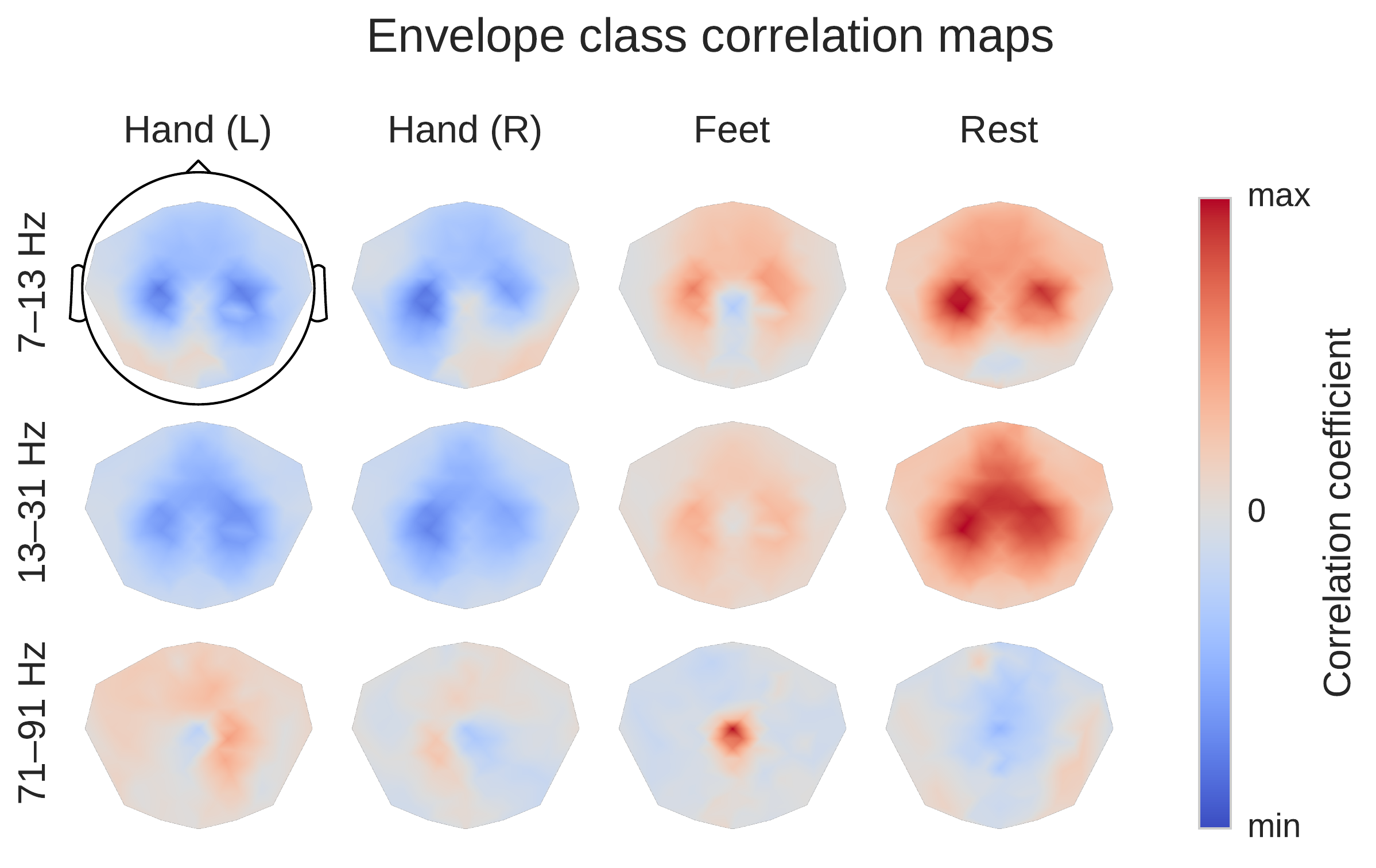
Fig. 24 Average over subjects from the High-Gamma Dataset. Colormaps are scaled per frequency band/row. This is a ConvNet-independent visualization. Scalp plots show spatial distributions of class-related spectral amplitude changes well in line with the literature. Figure from Schirrmeister et al. [2017].#
Before moving to ConvNet visualization, we examined the spectral amplitude changes associated with the different movement classes in the alpha, beta and gamma frequency bands. For that, we first computed the moving average of the squared envelope in narrow frequency bands via the Hilbert transform as a measure of the power in those frequency bands. Then we computed linear correlations of these moving averages with the class label. This results in frequency-resolved envelope-class label correlations.
We found the expected overall scalp topographies (see Fig. 24) to show physiologically plausible patterns. For example, for the alpha (7–13 Hz) frequency band, there was a class-related power decrease (anti-correlation in the class-envelope correlations) in the left and right pericentral regions with respect to the hand classes, stronger contralaterally to the side of the hand movement , i.e., the regions with pronounced power decreases lie around the primary sensorimotor hand representation areas. For the feet class, there was a power decrease located around the vertex, i.e., approx. above the primary motor foot area. As expected, opposite changes (power increases) with a similar topography were visible for the gamma band (71–91 Hz).
Amplitude Perturbation Visualizations#

Fig. 25 Input-perturbation network-prediction correlations for all frequencies for the deep ConvNet, per class. Plausible correlations, for example, rest positively, other classes negatively correlated with the amplitude changes in frequency range from 20 to 30 Hz. Figure from Schirrmeister et al. [2017].#
Our amplitude perturbation visualizations show that the network have learned to extract commonly used spectral amplitude features.We show three visualizations extracted from input-perturbation network-prediction correlations, the first two to show the frequency profile of the causal effects, the third to show their topography. Thus, first, we computed the mean across electrodes for each class separately to show correlations between classes and frequency bands. We see plausible results, for example, for the rest class, positive correlations in the alpha and beta bands and negative correlations in the gamma band in Fig. 25.

Fig. 26 Absolute input-perturbation network-prediction correlation frequency profile for the deep ConvNet. Mean absolute correlation value across classes. CSP binary decoding accuracies for different frequency bands for comparison, averaged across subjects and class pairs. Peaks in alpha, beta, and gamma band for input-perturbation network-prediction correlations and CSP accuracies. Figure from Schirrmeister et al. [2017].#
Then, second, by taking the mean of the absolute values both over all classes and electrodes, we computed a general frequency profile. This showed clear peaks in the alpha, beta, and gamma bands (Fig. 26). Similar peaks were seen in the means of the CSP binary decoding accuracies for the same frequency range.
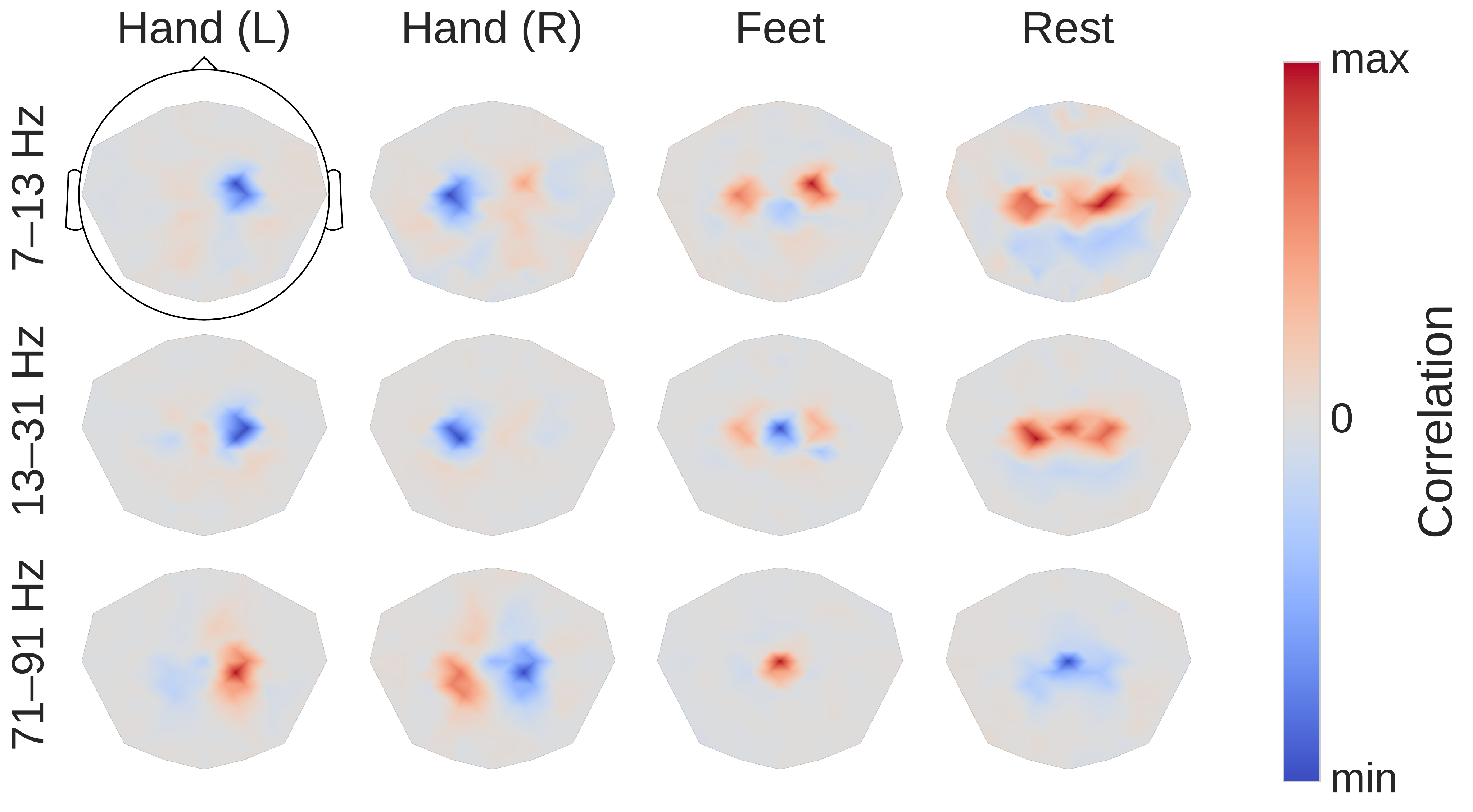
Fig. 27 Input-perturbation network-prediction correlation maps for the deep ConvNet. Correlation of class predictions and amplitude changes. Averaged over all subjects of the High-Gamma Dataset. Colormaps are scaled per scalp plot. Plausible scalp maps for all frequency bands, for example, contralateral positive correlations for the hand classes in the gamma band. Figure from Schirrmeister et al. [2017].#
Third, scalp maps of the input-perturbation effects on network predictions for the different frequency bands, as shown in Fig. 27, show spatial distributions expected for motor tasks in the alpha, beta and — for the first time for such a noninvasive EEG decoding visualization — for the high gamma band. These scalp maps directly reflect the behavior of the ConvNets and one needs to be careful when making inferences about the data from them. For example, the positive correlation on the right side of the scalp for the Hand (R) class in the alpha band only means the ConvNet increased its prediction when the amplitude at these electrodes was increased independently of other frequency bands and electrodes. It does not imply that there was an increase of amplitude for the right hand class in the data. Rather, this correlation could be explained by the ConvNet reducing common noise between both locations, for more explanations of these effects in case of linear models, see Interpretation and Limitations and [Haufe et al., 2014]. Nevertheless, for the first time in noninvasive EEG, these maps clearly revealed the global somatotopic organization of causal contributions of motor cortical gamma band activity to decoding right and left hand and foot movements. Interestingly, these maps revealed highly focalized patterns, particularly during hand movement in the gamma frequency range (Fig. 27, first plots in last row), in contrast to the more diffuse patterns in the conventional task-related spectral analysis as shown in Fig. 24.
Internal Representations of Amplitude and Phase#

Fig. 28 Mean phase and amplitude perturbation correlations over layers. Curves show mean perturbation correlation over all frequencies for each layer. Scales are different and written on the left and right y-axes. The error bars show the standard error over the subjects. Standard errors for phase and amplitude are similar, but much higher relatively in the amplitude correlation scale and therefore only visible there. In their respective scale, curves show a clearly inverse behavior over the layers with increasing amplitude correlations and decreasing phase correlations. Figure from Hartmann et al. [2018].#
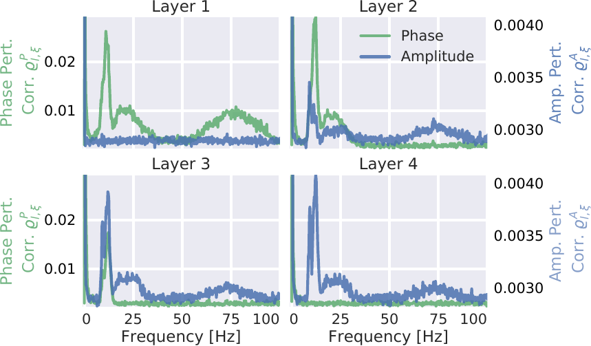
Fig. 29 Mean of absolute phase and amplitude perturbation correlations for individual frequencies. The two correlation types have different scales, denoted by the left and right y-axis. As in Fig. 28, a clearly inverse relation between amplitude and phase correlations is visible. This visualization additionally showed that alpha (7-13 Hz), beta (13-30 Hz), and high gamma (50-100 Hz) frequency ranges each have a specific layer in which their phase correlation vanishes and their amplitude correlation saturates (high gamma in layer 2, beta in layer 3, and alpha in layer 4). Figure from Hartmann et al. [2018].#
The perturbation analysis showed that the earlier layers represent more phase-specific features than later layers, while the later layers represent more phase-invariant amplitude features than the early layers. Fig. 28 shows the average absolute phase perturbation correlation and amplitude perturbation correlation over the 4 convolutional layers. The figure shows a clearly opposing development of their respective average values across layers, with increasing amplitude perturbation correlations and decreasing phase perturbation correlations.
The perturbation correlations for individual frequencies showed a strong phase perturbation correlation in the earlier layers 1 and 2 to phases in the alpha, beta, and high gamma range (see Fig. 29 ). The overall phase perturbation correlation was highest in layer 1 and gradually became lower over layers 2, 3, and 4. Interestingly, for each frequency band (alpha, beta, and high gamma), there was one specific layer in which the phase perturbation correlations vanished completely. Phase perturbation correlations for high gamma vanished in layer 2, correlations for beta vanished in layer 3, and correlations for alpha vanished in layer 4. This vanishing of phase correlations for high gamma in layer 2 could be observed in all subjects. For 4 subjects, alpha did already vanish together with beta in layer 3.
An opposite behavior could be observed for amplitude correlations. Notable phase insensitive amplitude perturbation correlations are only emerging in layer 2. Amplitude correlations of individual frequency bands peaked and saturated in the same layers in which the phase correlation vanished: High gamma amplitude perturbation correlation saturated in layer 2, beta in layer 3, and alpha in layer 4.
A potential underlying reason may be the use of max pooling with stride 3 after layers 1,2 and 3. The resulting temporal frequency resolutions of the intermediate representations when only taking into account the pooling strides are \(\frac{250 \textrm{Hz}}{3} \approx 83\textrm{Hz}\), \(\frac{250 \textrm{Hz}}{3^2} \approx 28\textrm{Hz}\) and \(\frac{250 \textrm{Hz}}{3^3} \approx 9\textrm{Hz}\). The corresponding Nyquist frequencies of approximately \(41.5\textrm{Hz}\), \(14\textrm{Hz}\) and \(4.5\textrm{Hz}\) seem to correspond to frequency cutoffs above which the network is no longer phase-sensitive. However, note that the network is in principle capable of retaining phase sensitivity even in the presence of max pooling by shifting temporal information to its channel dimension.
Maximally Activating Units#
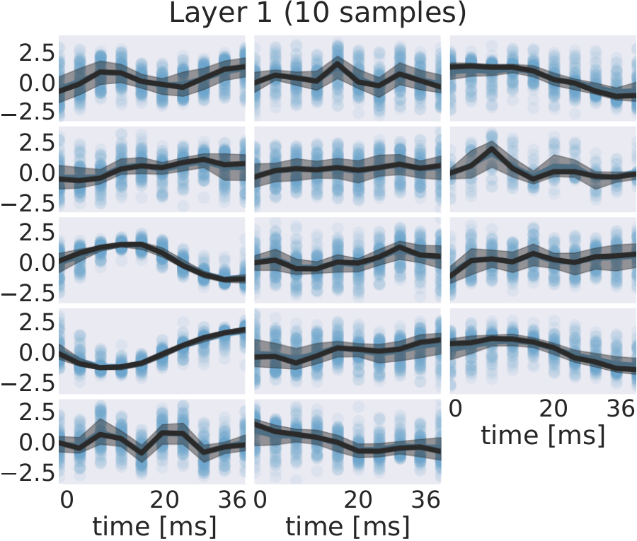
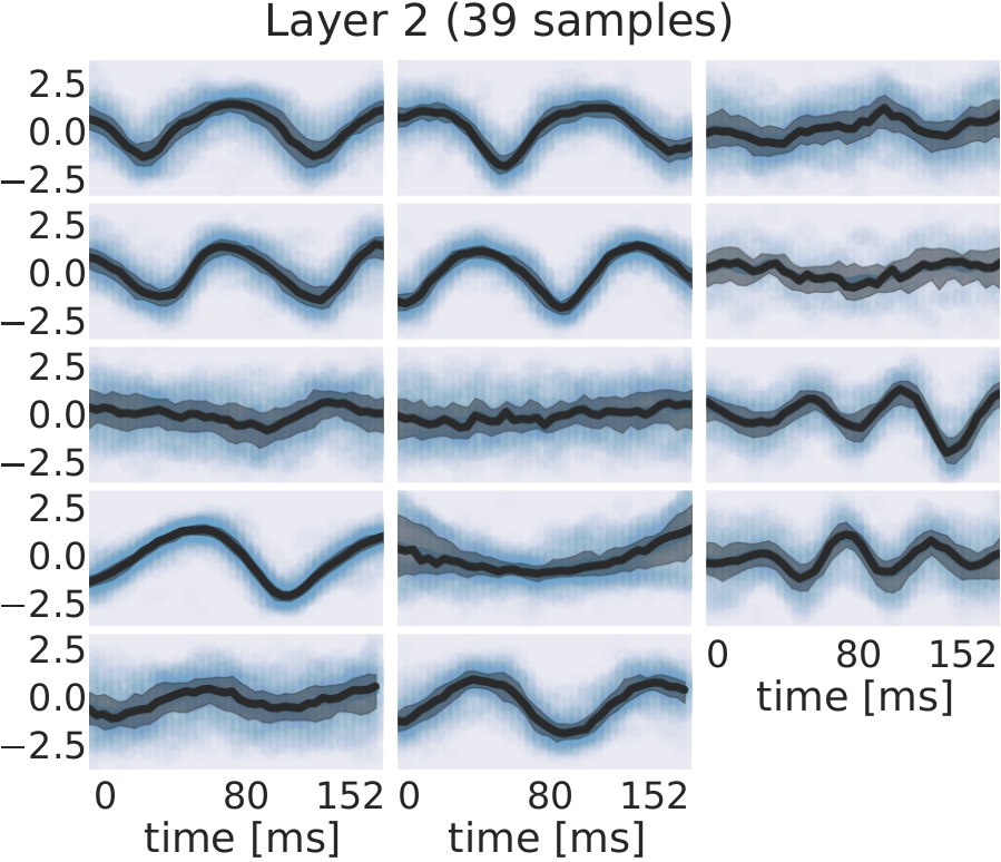
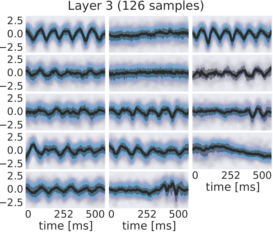
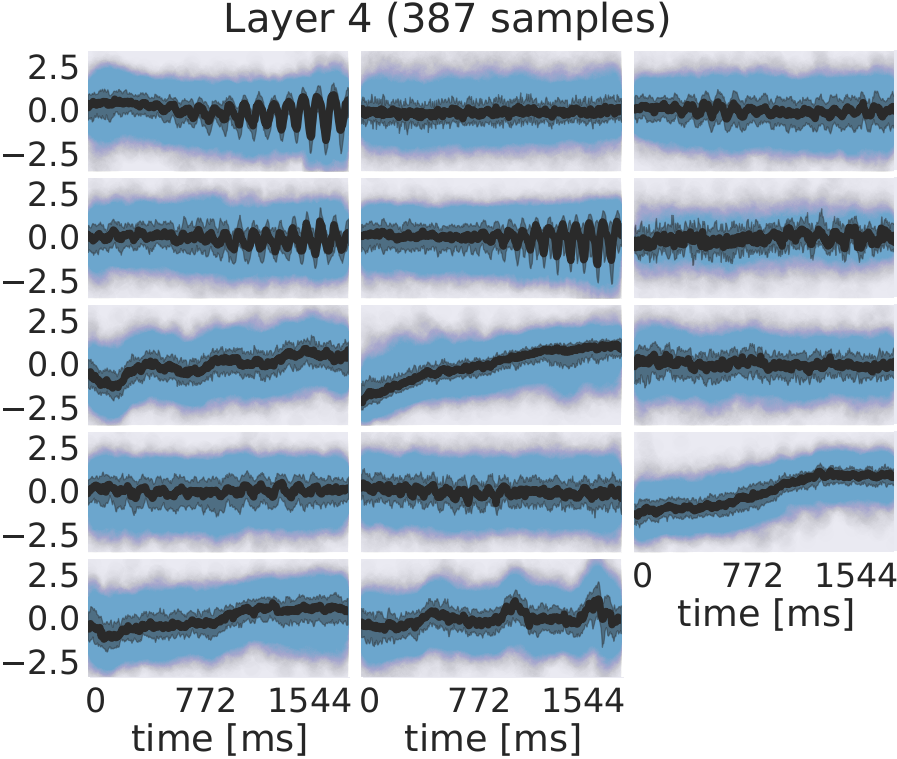
Fig. 30 EEG signals in most-activating input windows of one randomly sampled filter from each subject for each layer. Blue points are the standard scores of all most-activating input windows for a filter. Their median is shown in black and the interquartile range as a gray shaded area. Medians with respect to earlier layers often resemble parts of or complete sinusoids while medians in later layers resemble more complex patterns. Figure from Hartmann et al. [2018].#
In addition to examining how the individual layers respond to frequency-specific phase and amplitude, we were also interested in other characteristic features that might be learned by filters. To investigate other features than frequency-specific phase or amplitude of sinusoidal signals, we visually inspected the most-activating input windows of a filter and their median values for each timepoint. Fig. 30 shows the most-activating input windows of one randomly sampled filter for each subject and layer. We show each such set of most activating input windows here at a representative electrode.
For several filters, a clearly defined structure was present in the median. The median plots for layer 1 show several examples of sinusoidal shapes in different frequencies. Medians of higher frequencies were sharper and the variance across input windows is larger. Medians of layer 2 revealed several smooth alpha sinusoids, but also examples of beta waves. In addition to that, there were some flat medians without an easily interpretable periodicity or other temporal structure. In layer 3, there were mostly examples for alpha waves. For some medians in layer 4, more complex temporal patterns emerged. Those medians were relatively flat at the beginning of the input windows, but showed an oscillatory pattern with increasing amplitude in the later parts of the input windows. Also, the oscillatory patterns in some examples resembled mu waves more closely than pure sinusoids. Such patterns were found in several subjects.
Braindecode#
Work performed for this study also later led to the creation of the open-source EEG deep learning library Braindecode, now with contributions from multiple research groups and available at braindecode/braindecode.
Open questions
How well do ConvNets perform on other decoding tasks?
Do they work on tasks where oscillatory features are less important?
Do they work on non-trial based tasks like decoding pathology?