Invertible Networks#
Invertible networks can help understand learned discriminative features in the EEG
Class prototypes can be visualized
Per-electrode prototypes may be even more interpretable
Additionally, a small interpretable network may allow further insights
Invertible networks are networks that are invertible by design, i.e., any network output can be mapped back to a corresponding input bijectively [Dinh et al., 2015, Dinh et al., 2016, Ho et al., 2019, Kingma and Dhariwal, 2018, Rezende and Mohamed, 2015]. The ability to invert any output back to the input enables different interpretability methods and furthermore allows training invertible networks as generative models via maximum likelihood.
This chapter starts by explaining invertible layers that are used to design invertible networks, proceeds to detail training methodologies for invertible networks as generative models or classifiers, and goes on to outline interpretability techniques that help reveal the learned features crucial for their classification tasks. \(\require{color}\) \(\definecolor{commentcolor}{RGB} {70,130,180}\)
Invertible Layers#
Invertible networks use layers constructed specifically to maintain invertibility, thereby rendering the entire network structure invertible. Often-used invertible layers are coupling layers, invertible linear layers and activation normalization layers [Kingma and Dhariwal, 2018].
Coupling layers split a multidimensional input \(x\) into two parts \(x_1\) and \(x_2\) with disjoint dimensions and then use \(x_2\) to compute an invertible transformation for \(x_1\). Concretely, for an additive coupling layer, the forward computation is:
\( \begin{align*} y_1 &= x_1 + f(x_2) && \color{commentcolor}{\text{Compute } y_1 \text{ from } x_1 \text{ and arbitrary function f of } x_2} \\ y_2 &= x_2 && \color{commentcolor}{\text{Leave } x_2 \text{ unchanged}} \\ \end{align*} \)
The inverse computation is:
\( \begin{align*} x_1 &= y_1 - f(y_2) && \color{commentcolor}{\text{Invert to } x_1 \text{ using unchanged } y_2=x_2} \\ x_2 &= y_2 && \color{commentcolor}{x_2 \text{ was unchanged}}\\ \end{align*} \)
For the splitting of the dimensions in a timeseries, there are multiple ways, such as using the even time indices as \(x_1\) and all the odd time indices as \(x_2\) or using difference and mean between two neighbouring samples (akin to one stage of a Haar Wavelet). The function \(f\) is usually implemented by a neural network, in our cases it will be small convolutional networks. Instead of addition any other invertible function can be used, affine transformation are commonly used, where \(f\) produces translation and scaling coefficients \(f_t\) and \(f_s\):
\( \begin{align*} y_1 &= x_1 \cdot f_s(x_2) + f_t(x_2) && \text{ } y_2=x_2 && \color{commentcolor}{\text{Affine Forward }} \\ \\ x_1 &= \frac{(y_1 - f_t(y_2))}{f_s(y_2)} && \text{ } x_2=y_2 && \color{commentcolor}{\text{Affine Inverse}} \\ \end{align*} \)
Invertible linear layers compute an invertible linear transformation (an automorphism) of their input. Concretely they multiply a \(d\)-dimensional vector \(\mathbf{x}\) with a \(dxd\)-dimensional matrix \(W\), where \(W\) has to be invertible, i.e., have nonzero determinant.
\( \begin{align*} y&=W \mathbf{x} && \color{commentcolor}{\text{Linear Forward }} \\ x&=W^{-1} \mathbf{y} && \color{commentcolor}{\text{Linear Inverse}} \\ \end{align*} \)
For multidimensional arrays like feature maps in a convolutional network, these linear transformations are usually done per-position, as so-called invertible 1x1 convolutions in the 2d case.
Activation normalization layers perform an affine transformation with learned parameters with \(s\) and \(t\) learned scaling and translation parameters (independent of the input \(x\)):
\( \begin{align*} y&=x \cdot{s} + t && \color{commentcolor}{\text{ActNorm Forward }} \\ x&=\frac{y - t}{s} && \color{commentcolor}{\text{ActNorm Inverse}} \\ \end{align*} \)
These have also been used to replace batch normalization and are often initialized data-dependently to have standard-normalized activations at the beginning of training.
Generative Models by Maximizing Average Log Likelihood#
Invertible networks can also be trained as generative models via maximizing the average log likelihood. In this training, the network is optimized to maximize the average log probabilities of the training inputs, which is equivalent to minimizing the Kullback-Leibler (KL) divergence between the training distribution and the learned model distribution [Theis et al., 2016]. Invertible networks assign probabilities to training inputs \(x\) by mapping them to a latent space \(z=f(x)\) and computing their probabilities under a predefined prior \(p_z(z)\) in that latent space. For real-valued inputs, one has to account for quantization and volume change to ensure this results in a proper probability distribution \(p_x\) in the input space. Quantization refers to the fact that training data often consists of quantized measurements of underlying continuous data, e.g. digital images can only represent a distinct set of color values. Volume change refers to how the invertible networks’ mapping function \(f\) expands or squeezes volume from input space to latent space.
(De)quantization#
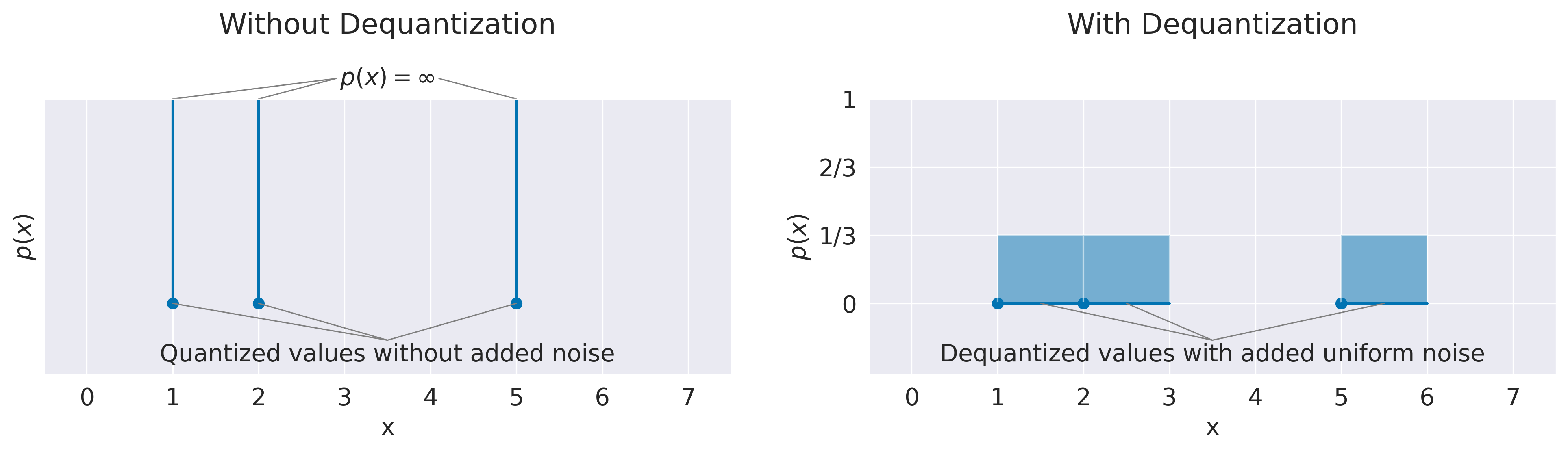
Fig. 14 Density-maximizing distributions without and with dequantization. Examples show result of fitting quantized values like discrete integer color values with a continuous probability distribution. Example training distributions have 3 data points at \(x_1=1\), \(x_2=2\) and \(x_3=5\). On the left, fitting quantized values directly leads to a pathological solution as the learned distribution \(p\) can assign arbitrarily high probability densities on the data points. On the right, adding uniform noise \(U(0,1)\) to the datapoints leads to a distribution that also recovers the correct discrete distribution, that means integrating over the probability densities in the volume of each point leads to \(P(x_i)=\frac{1}{3}\).#
Often, training data for neural networks consists of quantized measurements like discrete integer color values from 0 to 255, which are mapped to real-world floating point numbers for training. Naively maximizing the average log probability densities of these quantized values with a continuous probability distribution would lead to pathological behavior as the quantized training data points do not cover any volume. Hence it would be possible for the learned distribution to assign infinitely high probability densities to individual data points, see Fig. 14 for an illustration.
Hence, one needs to “dequantize” the data such that each datapoint occupies volume in the input space [Dinh et al., 2016, Ho et al., 2019]. The simplest way here is to add uniform noise to each data point with a volume corresponding to the gap between two data points. For example, if the 256 color values are mapped to 256 floating values between 0 and 1, one may add uniform noise \(u\sim(0,\frac{1}{256})\) to the inputs. Then the KL-divergence between the dequantized continuous distribution and the learned continuous distribution is upper bounded by the KL-divergence between the underlying discrete distribution and the learned discrete distribution obtained by integrating over the noise samples for each input [Theis et al., 2016]. Since in our case, we are not primarily interested in the exact performance as a generative model in terms of number of bits, we simply add gaussian noise with a fixed small standard deviation \(N(0,0.005I)\) during training.
Volume Change#
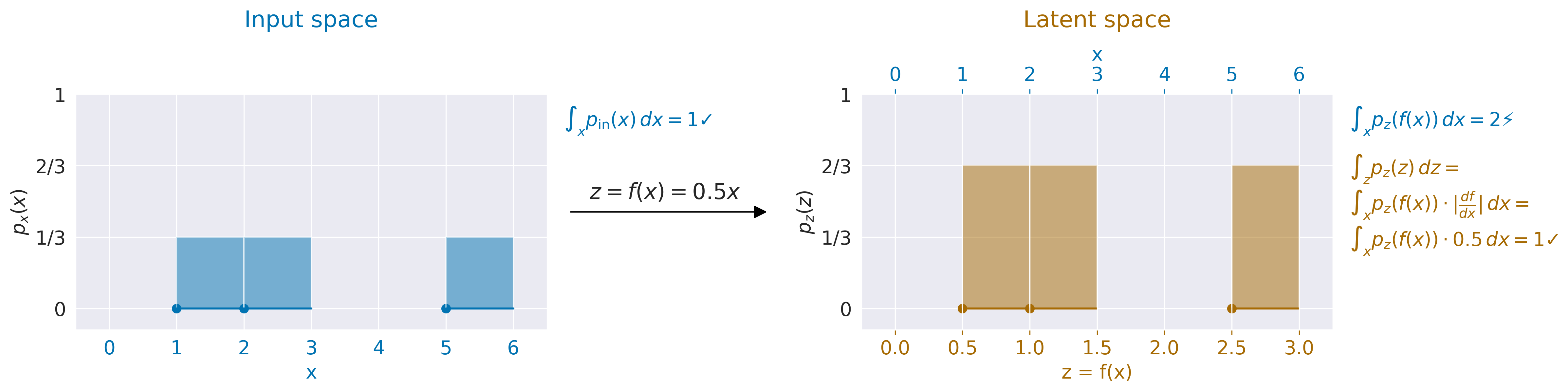
Fig. 15 Computing probability densities accounting for volume changes by a function. Input \(x\) with probability distribution \(p_\text{x}(x)\) on the left is scaled by 0.5 to \(z=f(x)=0.5x\) with probability distribution \(p_\text{z}(z)\) on the right. Naively integrating \(p_\text{z}(f(x))\) over x would lead to a non-valid probability distribution with \(\int_x p_\mathrm{z}(f(x)) \, dx=2\). To get the prober probability densities in input space from \(p_\text{z}(z)\), one has to multiply with the volume changes, in this case the scaling factor of the mapping \(f(x)\) from x to z, giving \(p_\text{x}(x)=p_\mathrm{z}(f(x)) \cdot \frac{df}{dx}=p_\mathrm{z}(f(x))\cdot 0.5\) which correctly integrates to 1.#
In addition, for these probability densities in latent space to form a valid probability distribution in the input space, one has to account for how much the network’s mapping function squeezes and expands volume. Otherwise, the network can increase densities by squeezing all the inputs closely together in latent space, see also Fig. 15 for a onedimensional example. To correctly account for the volume change during the forward pass of \(f\) one needs to multiply the probability density with the volume change of \(f\), descreasing the densities if the volume is squeezed from input to latent space and increasing it if the volume is expanded. As the volume change at a given point \(x\) is given by the absolute determinant of the jacobian of f at that point \(\det \left( \frac{\partial \mathbf{f}}{\partial \mathbf{x}} \right)\), the overall formula looks like this:
\(p(x) = p_\textrm{z}(f(x)) \cdot | \det \left( \frac{\partial \mathbf{f}}{\partial \mathbf{x}} \right)|\)
Or in log-densities:
\(\log p(x) = \log p_\textrm{z}(f(x)) + \log |\det \left( \frac{\partial \mathbf{f}}{\partial \mathbf{x}} \right)|\)
Generative Classifiers#
Invertible networks trained as class-conditional generative models can also be used as classifiers. Class-conditional generative networks may be implemented in different ways, for example with a separate prior in latent space for each class. Given the class-conditional probability densities \(p(x|c_i)\), one can obtain class probabilities via Bayes formula as \(p(c_i|x)=\frac{p(x|c_i)}{\sum_jp(x|c_j)}\).
Pure class-conditional generative training may yield networks that perform badly as classifiers. One proposed reason is the relatively small reduction in optimal average log likelihood loss obtainable from providing the class label to the network for high-dimensional inputs, often much smaller than typical differences between two runs of the same network [Theis et al., 2016]. The reduction in the optimal average log likelihood loss through providing the class label can be derived from a compression perspective. According to Shannon’s theorem, more probable inputs need less bits to encode than less probable inputs, or more precisely \(\textrm{Number of bits needed}(x) = \log_2 p(x)\). How many of these bits are needed for the class label in case it is not given? To distinguish between n classes, one needs only \(\log_2(n)\) bits, so in case of binary pathology classification, only 1 bit is needed. Therefore the optimal class-conditional model will only be 1 bit better than the optimal class-independent model. However, the inputs themselves typically need at least 1 bit per dimension, so already, a 21 channel x 128 timepoints EEG-signal may need at least 2688 bits to encode. Hence, the class encoding contributes very little to the overall encoding size and maximum likelihood loss. In contrast, the loss difference between two training runs of the same network will typically be at least one to two orders of magnitude larger. Still, in practice, the gains from using a class-conditional model, by e.g., using a separate prior per class in latent space, are often larger, but it is not a priori clear if the reductions in loss from exploiting the class label are high enough to result in a good classification model.
Various methods have been proposed to improve the performance of using generative classifiers. For example, people have fixed the per-class latent gaussian priors so that they retain the same distance throughout training [Izmailov et al., 2020] or added a classification loss term \(L_\textrm{class}(x,c_i)=-\log p(c_i|x) = -\log \frac{p(x|ci)}{\sum_j p(x|cj)}=-\log \frac{e^{\log p(x|ci)}}{\sum_j e^{\log p(x|cj)}}=-\log \left( \mathrm{softmax}\left({\log p(x|c_i)}\right) \right)\) to the training loss[Ardizzone et al., 2020]. In our work, we experimented with adding a classification loss term to the training, and also found using a learned temperature before the softmax helps the training, so leading to:
\( \begin{align*} L_\textrm{class}(x,c_i,t)&= -\log \frac{e^{\frac{\log p(x|ci)}{t}}}{\sum_j e^{\frac{\log p(x|cj)}{t}}}=-\log \left( \mathrm{softmax}\left({\frac{\log p(x|c_i)}{t}}\right) \right) \\ \end{align*} \)
Our overall training loss is simply a weighted sum of generative loss and classification loss:
\( \begin{align*} L(x,c_i,t)&= L_\textrm{class}(x,c_i,t) + L_\textrm{gen}(x,c_i) &= -\log \left( \mathrm{softmax}\left({\frac{\log p(x|c_i)}{t}}\right) \right) - \alpha \log p(x|ci)\\ \end{align*} \)
where we choose the hyperparameter \(\alpha\) as the inverse of the number of dimensions \(\alpha=\frac{1}{\textrm{Number of dimensions of x}}\).
Invertible Network for EEG Decoding#
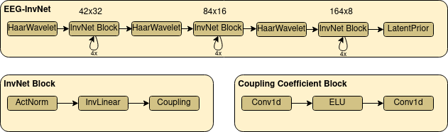
Fig. 16 EEG-InvNet architecture. Our EEG-InvNet architecture consists of three stages that operate at sequentially lower temporal resolutions. Input is two seconds of 21 electrodes at 64 Hz so 21x128 dimensions. These are downsampled using Haar Wavelets to 42x32 for the first, 84x16 for the second and 164x8 for the last stage. One stage consists of 4 blocks, each block has an activation normalization, an invertible linear and a coupling layer. The activation normalization and invertible linear layer act on the channel dimension, so perform the same operation across channels on timepoint in the feature map. The coupling layer uses two convolutions with an exponential linear unit activation inbetween.#
We designed an invertible network named EEG-InvNet for EEG Decoding using invertible components used in the literature, primarily from the Glow architecture [Kingma and Dhariwal, 2018]. Our architecture consists of three stages that operate on sequentially lower temporal resolutions. Similar to Glow, the individual stages consists of several blocks of Activation Normalization, Invertible Linear Channel Transformations and Coupling Layers, see Fig. 16. Between each stage, we downsample by computing the mean and difference of two neighbouring timepoints and moving these into the channel dimension. Unlike Glow, we keep processing all dimensions throughout all stages, finding this architecture to reach competitive accuracy on pathology decoding. We use one gaussian distribution per class in the latent space. We experimented with affine and additive coupling layers, and report results for additive layers as the restricted expressiveness may make them easier to interpret.
Class Prototypes#
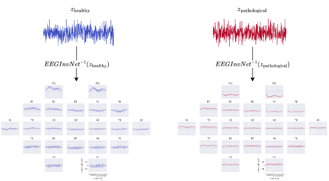
Fig. 17 EEG-InvNet class prototypes. Class prototypes are synthesized by inverting the means \(z_\mathrm{healthy}\) and \(z_\mathrm{pathological}\) of the per-class gaussian distributions.#
In our first visualization, we show the inputs resulting from inverting the means of the gaussian distributions for each class (see Fig. 17) . These can be seen as prototypical examples of each class and may give hint about the discriminative features that have been learned. As these are only single examples, they need to be interpreted cautiously. For example, individual features within the examples may have a variety of relationships with the actual prediction function. Consider if a prototype contains a large alpha-band oscillation at two electrodes, then these may be indepedendently predictive predictive of that class or only in combination or even only in some combination with other features. Nevertheless, the prototypes can already suggest potential discriminative features for further investigation.
Per-Electrode Prototypes#
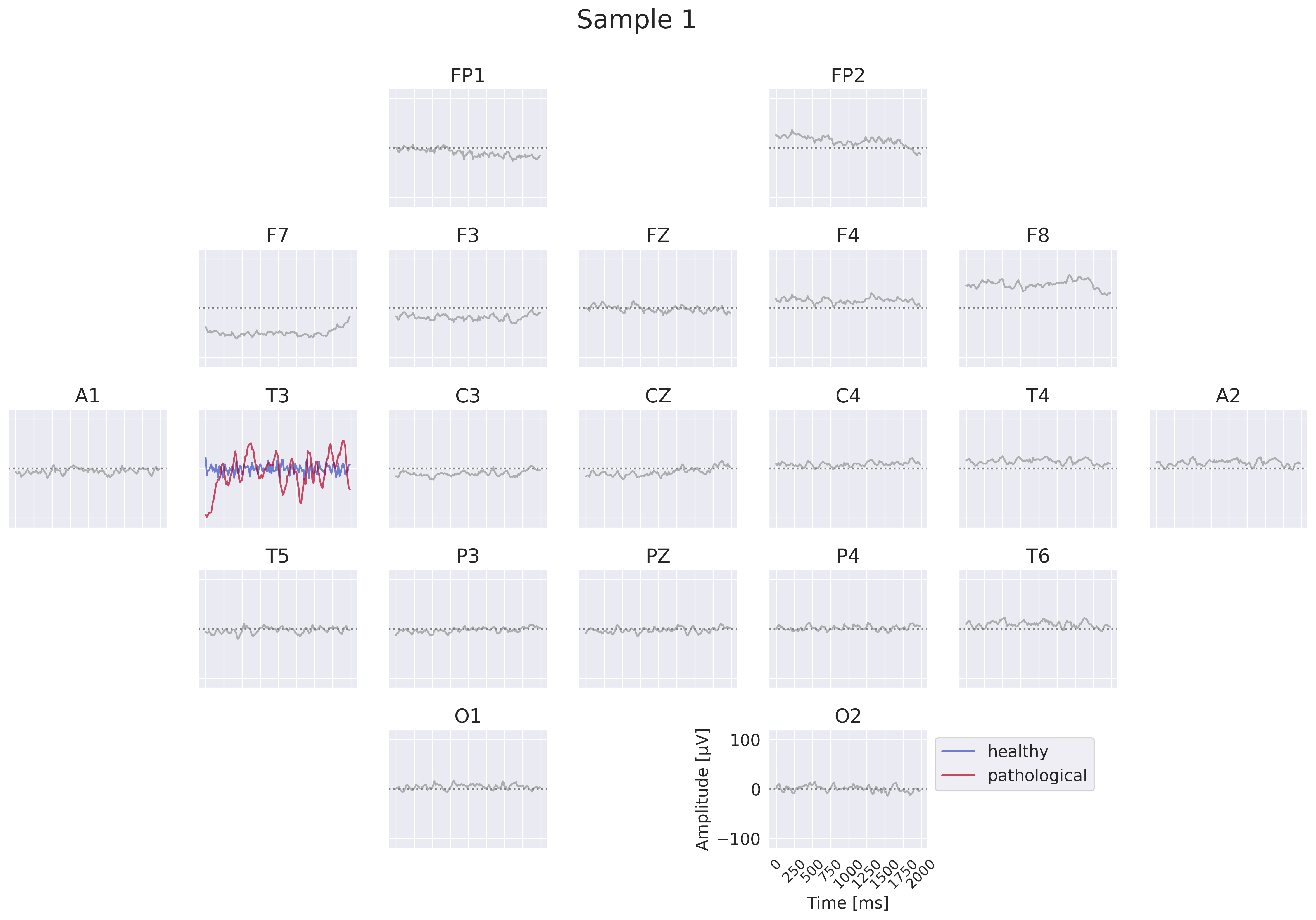
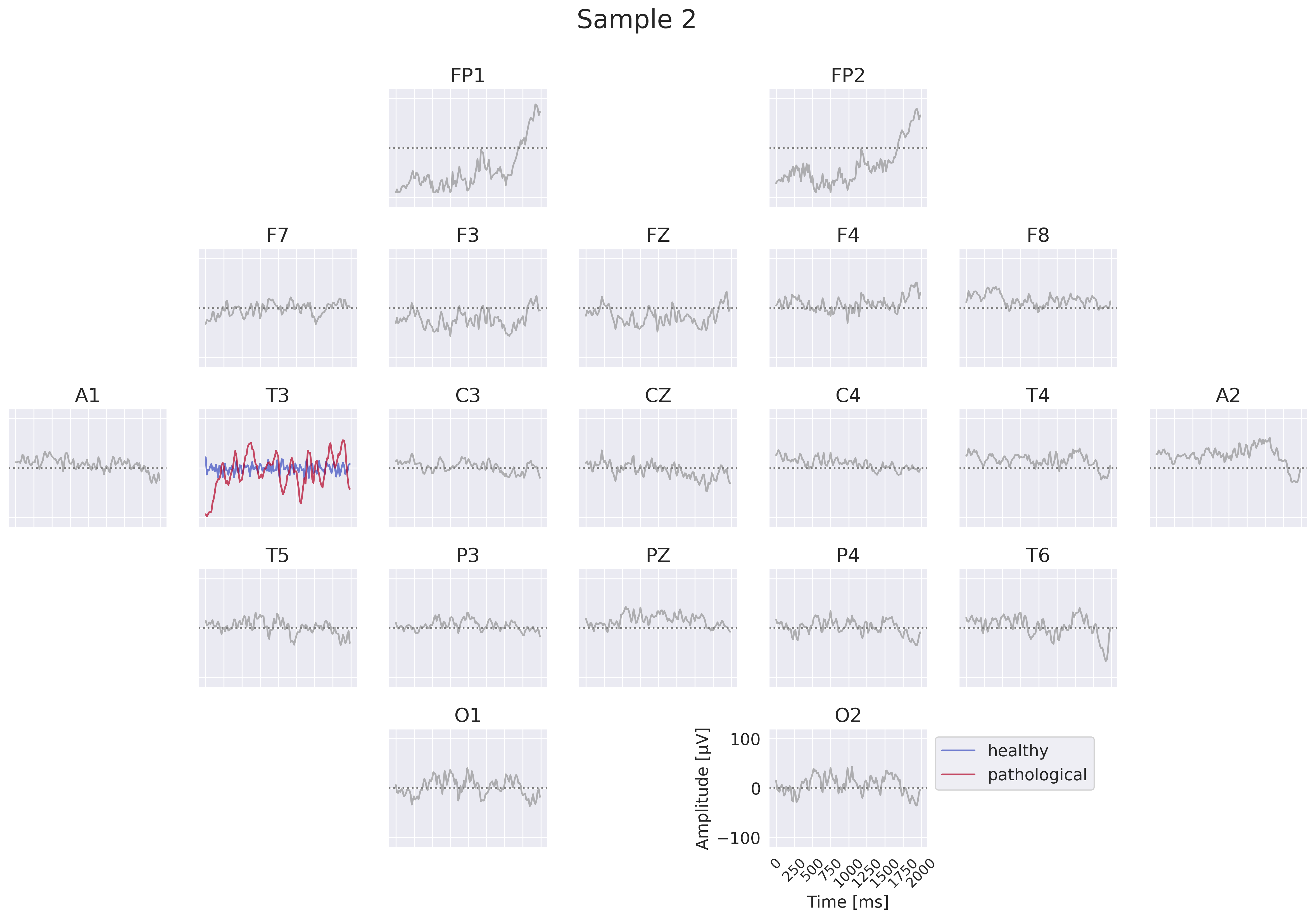
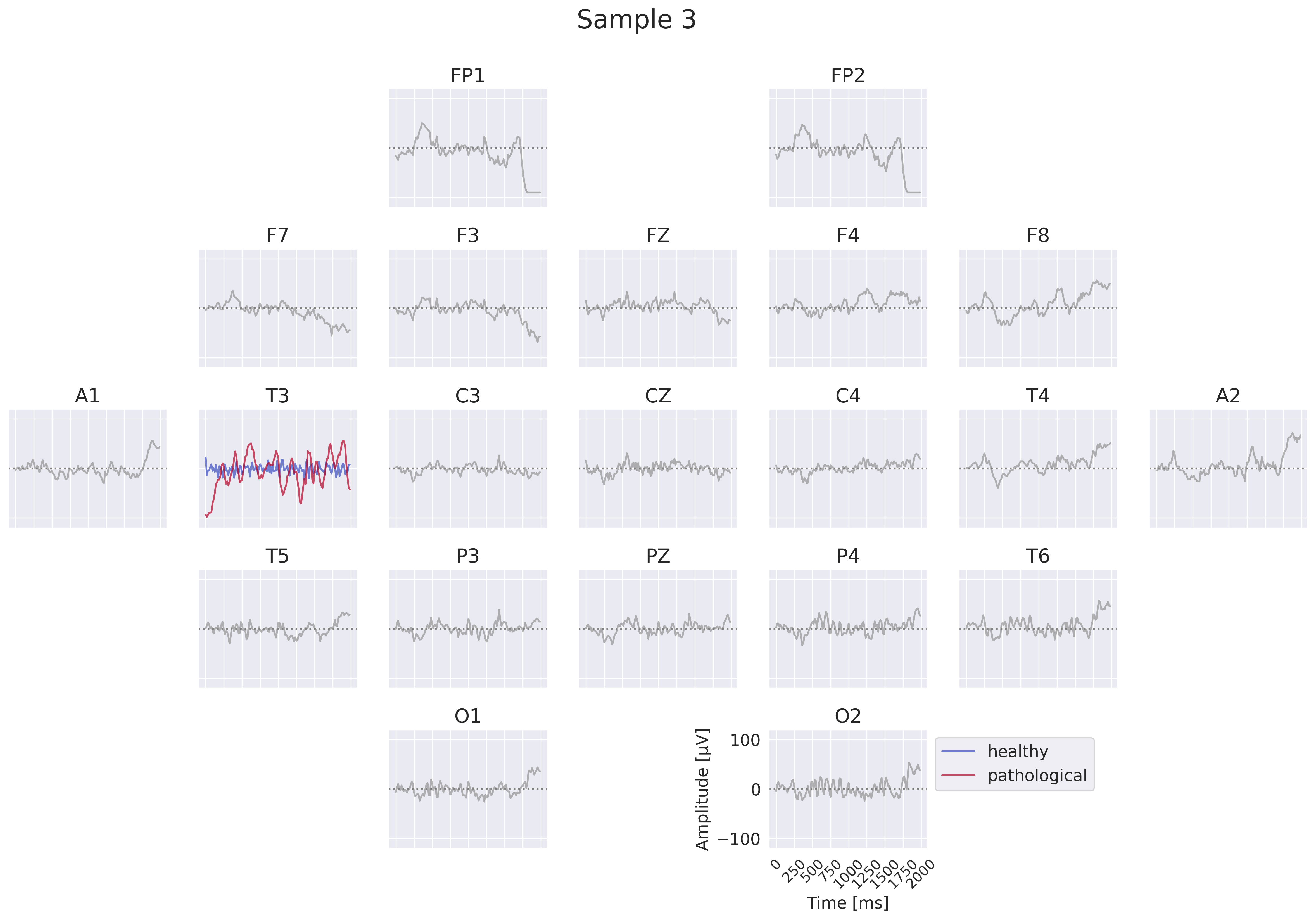
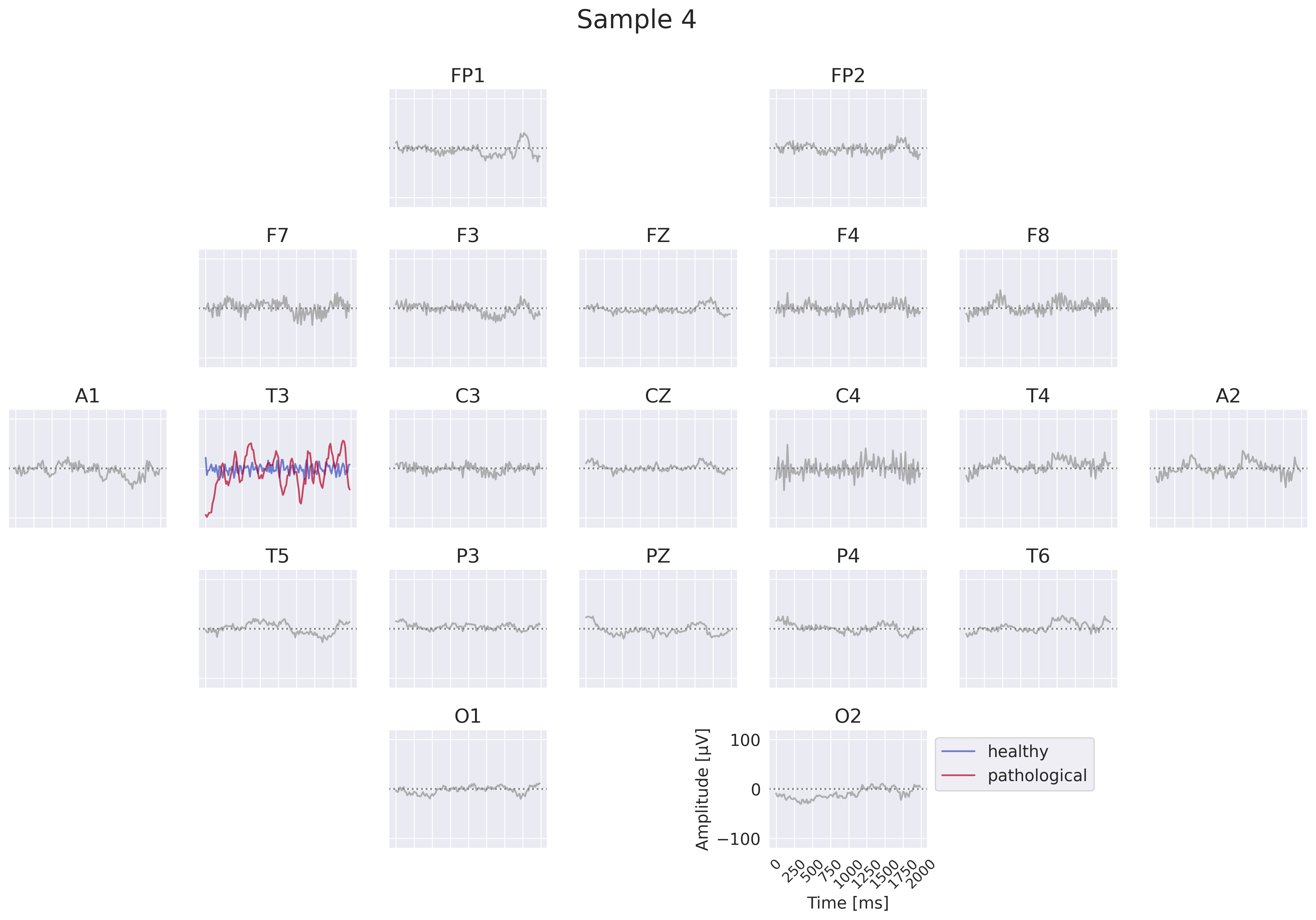
Fig. 18 EEG-InvNet per-electrode class prototypes. For getting per-electrode prototypes, class-specific signals for one electrode are synthesized while signals at other electrodes are sampled from training data. In the example, prototypes for T3 for the healthy and pathological class are learned, four samples for remaining electrodes are shown. In practice, a much larger number of samples would be used. Class signal probabilities are marginalized over the non-optimized channels as explained in text.#
One way to get more interpretable prototypes is to synthesize them per electrode. Here, we synthesize a signal \(x^*_{e_k}\) for a specific electrode \(e_k\) such that the class prediction is high for one class, independent of the signals at the other electrodes (see Fig. 18). So for electrode \(e_k\) and class \(c_i\), we aim to optimize the signal \(x^*_{e_k}\) by maximizing the marginals \(p(x^*_{e_k}|c_i)=\int p(x|c_i;x_{e_k}=x^*_{e_k}) dx\) (generative loss) and \(p(c_i|x^*_{e_k})=\frac{p(x^*_{e_k}|c_i)}{\sum_j p(x^*_{e_k}|c_j)}\) (classification loss). To approximate this, we sample \(n\) signals \(x_l\) of the training distribution and replace the signal \(x_{l,e_k}\) of the electrode \(e_k\) we are synthesizing by the optimized \(x^*_{e_k}\). This leads to \(p(x^*_{e_k}|c_i)\approx\sum_{l=1}^n p(x_l|c_i;x_{l,e_k}=x^*_{e_k})\). While being only a coarse approximation, this already yields insightful visualizations. For the classification loss, when computing \(p(c_i|x^*_{e_k})\), we found it helpful to first divide the log probabilities \(\log p(x_l|c_i;x_{l,e_k}=x^*_{e_k})\) by the learned temperature \(t\) of the classifier: \(\log p_\mathrm{clf}(x^*_{e_k}|c_i)=\mathrm{logsumexp}\left(\frac{\log p(x_l|c_i;x_{l,e_k}=x^*_{e_k})}{t}\right)\). Otherwise, \(\sum_n p(x_n|c_i;x_{n,e_k}=x^*_{e_k})\) may be dominated by just a few samples when computing \(p(c_i|x^*_{e_k})\). We only apply this for the classification loss \(p(c_i|x^*_{e_k})\), not the generative loss \(p(x^*_{e_k}|c_i)\).
EEG-CosNet#
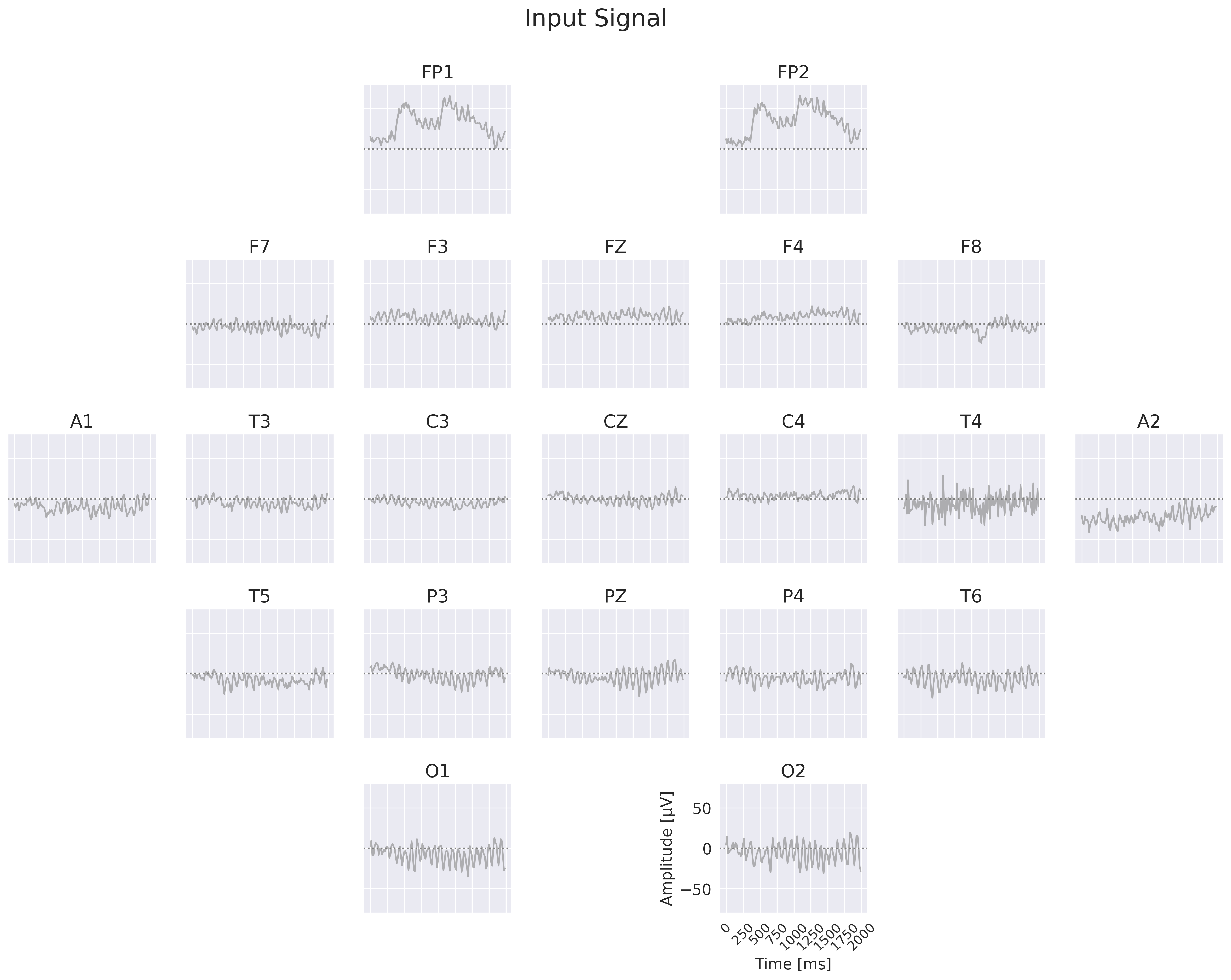
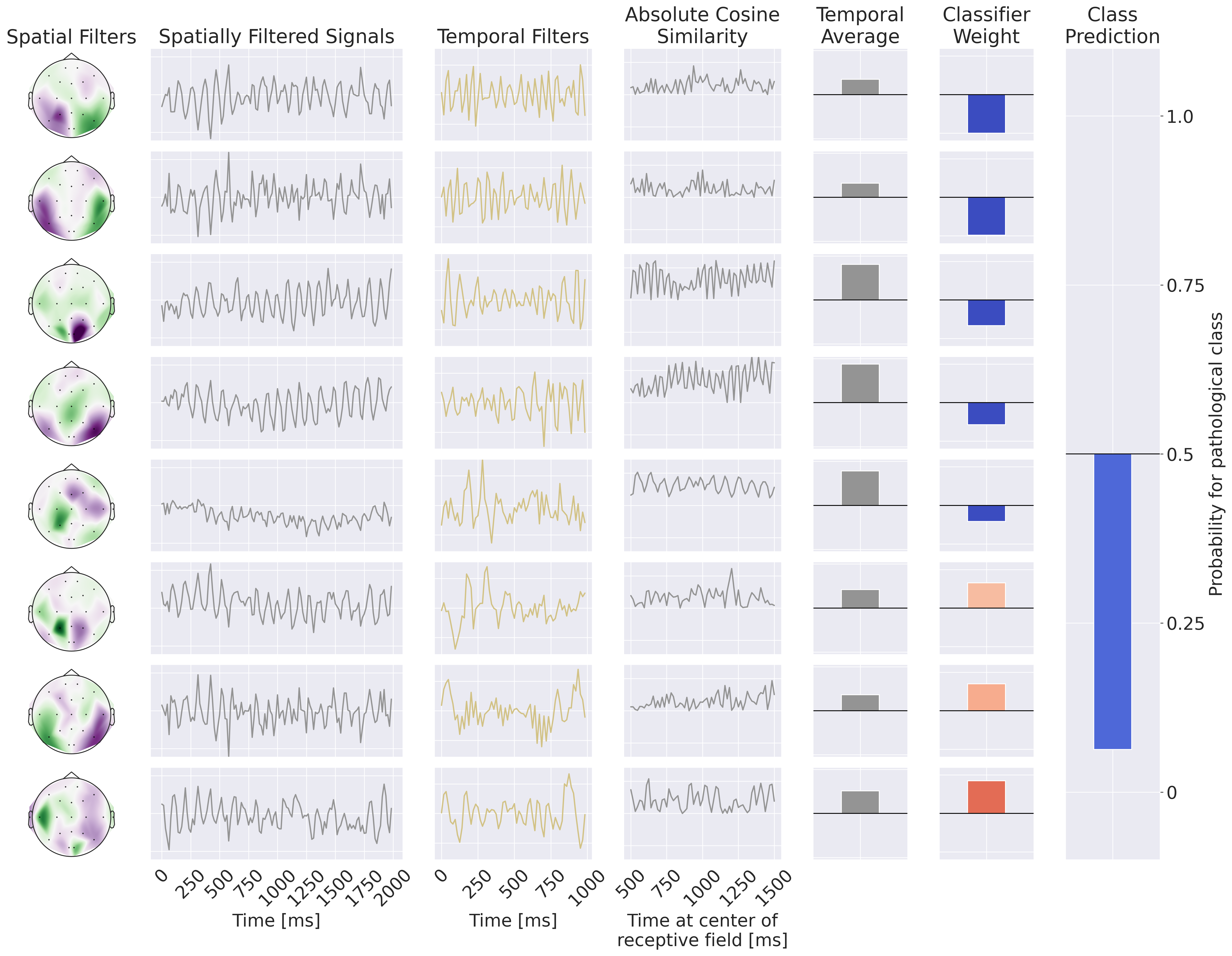
Fig. 19 Example Processing of the EEG-CosNet. Example EEG input on the left, then processing steps on the right: spatial filtering, absolute cosine similarity with temporal filters, temporal averaging, then weighting with linear classifier weights for class prediction. Note the EEG-CosNet in this visualization only uses 8 filters, whereas later we will use 64 filters.#
Finally, we also implemented a small convolutional network EEG-CosNet that we designed to be directly interpretable. We tried to distill the trained EEG-InvNet into the EEG-CosNet by training the EEG-CosNet using the EEG-InvNet class probabilities as the targets for the classification loss \(L_\textrm{class}\). Our EEG-CosNet consists of just three steps (see Fig. 19 for an example computation):
Spatial Filtering
\( \begin{align*} h_1 &= W_s^Tx && \color{commentcolor}{\text{Apply learnable spatial filter weights } W_s \text{ to inputs }} \\ \end{align*} \)
Absolute Temporal Cosine Similarity with Temporal Filters
\( \begin{align*} h_2 &= |\mathrm{moving\_cos\_sim}(h_1, \mathrm{temporal\_filters})| && \color{commentcolor}{\text{Moving absolute cosine similarity with temporal filters, one temporal filter per spatial filter }} \\ h_3 &=\frac{\sum_t (h_2)}{n_\mathrm{times}} && \color{commentcolor}{\text{Average over timepoints in trial}} \\ \end{align*} \)
Classification
\( \begin{align*} h_4 &= W_c^Th_3 && \color{commentcolor}{\text{Apply learnable classification weights } W_c \text{ on these spatiotemporal features }} \\ p(\mathrm{pathological}|h_4) &= \frac{1}{1 + \sum_j e^-h_{4}} && \color{commentcolor}{\text{Take the sigmoid to compute probability of pathological class}} \\ \end{align*} \)
Steps 1 and 2 yield spatiotemporal patterns that can be visualized as waveforms and scalp plots, and that are weighted by the linear classifier for the respective classes. We chose cosine similarity to ensure that high output values correspond to spatially filtered signals that resemble the corresponding temporal filter. The spatial filter weights and linear classifier weights can be made even more interpretable through transforming the discriminative weights into generative patterns by multiplying them with the covariance of the electrodes/averaged absolute cosine similarities after training, see Haufe et al. [2014] for a discussion on this technique. We use 64 spatiotemporal filters with temporal length 64 corresponding to one second at 64 Hz.
Open Questions
How well can the EEG-InvNet perform on EEG Pathology decoding?
What features can the EEG-InvNet reveal?
How well can the EEG-CosNet approximate the EEG-InvNet?
What features can the EEG-CosNet reveal?