Prior Work

Prior to our work, research on deep-learning-based EEG decoding was limited

• Few studies compared to published feature-based decoding results

• Most EEG DL architectures had only 1-3 convolutional layers and included fully-connected layers with many parameters

• Most work only considered very restricted frequency ranges

• Most studies only compared few design choices and training strategies

Prior to 2017, when the first work presented in this thesis was published, there was only limited literature on EEG decoding with deep learning. In this chapter, I outline what decoding problems, input representations, network architectures, hyperparameter choices and visualizations were evaluated in prior work. This is based on the literature research that we presented in Schirrmeister et al. [2017].

Decoding Problems and Baselines

Table 1 Decoding problems in deep-learning EEG decoding studies prior to our work. Studies with published baseline compared their decoding results to an external baseline result published by other authors.

Decoding problem	Number of studies	With published baseline
Imagined or Executed Movement	6	2
Oddball/P300	5	1
Epilepsy-related	4	2
Music Rhythm	2	0
Memory Performance/Cognitive Load	2	0
Driver Performance	1	0

The most widely studied decoding problems were movement-related decoding problems such as decoding which body part (hand, feet etc.) a person is moving or imagining to move (see Table 1). From the 19 studies we identified at the time, only 5 compared their decoding results to an external published baseline result, limiting the insights about deep-learning EEG decoding performance. We therefore decided to compare deep-learning EEG decoding to a strong feature-based baseline (see Filter Bank Common Spatial Patterns and Filterbank Network) on widely researched movement-related decoding tasks.

Input Domains and Frequency Ranges

Show code cell source Hide code cell source

import matplotlib
import matplotlib.pyplot as plt
from matplotlib import cm
import seaborn
import numpy as np
import re
from myst_nb import glue
seaborn.set_palette('colorblind')
seaborn.set_style('darkgrid')
import re

%matplotlib inline
%config InlineBackend.figure_format = 'png'
#matplotlib.rcParams['figure.figsize'] = (12.0, 1.0)
matplotlib.rcParams['font.size'] = 14
a = np.array(['Time,  8–30 Hz ', 'Time, 0.1–40 Hz ', 'Time, 0.05–15 Hz ',
       'Time, 0.3–20 Hz ', 'Frequency, 6–30 Hz ', ' Frequency, 0–200 Hz ',
       'Time,  1–50 Hz ', ' Time,  0–100 HZ ',
       'Frequency, mean amplitude for 0–7 Hz, 7–14 Hz, 14–49 Hz ',
       'Time, 0.5–50 Hz ', 'Time,  0–128 Hz ',
       ' Frequency, mean power for 4–7 Hz, 8–13 Hz, 13–30 Hz ',
       'Time, 0.5–30Hz ', 'Time, 0.1–50 Hz ',
       'Frequency, 4–40 Hz, using FBCSP ',
       ' Time and frequency evaluated, 0-200 Hz ', 'Frequency, 8–30 Hz ',
       'Time, 0.15–200 Hz ', ' Time, 0.1-20 Hz '])
domain_strings = [s.split(',')[0] for s in a]
start_fs = [float(re.sub(r'[a-z ]+',r'', re.split(r'[–-–-]'," ".join(s.split(',')[1:]))[0])) for s in a]
end_fs = [float(re.sub(r'[a-z HZFBCSP]+',r'', re.split(r'[–-–-]'," ".join(s.split(',')[1:]))[1])) for s in a]
domain_strings = np.array(domain_strings)
start_fs = np.array(start_fs)
end_fs = np.array(end_fs)

freq_mask = np.array(['freq' in s.lower() for s in domain_strings])
time_mask = np.array(['time' in s.lower() for s in domain_strings])

fig = plt.figure(figsize=(8,4))
rng = np.random.RandomState(98349384)
color = seaborn.color_palette()[0]
i_sort = np.flatnonzero(time_mask)[np.argsort(end_fs[time_mask])]
for i, (d,s,e) in enumerate(zip(
        domain_strings[i_sort], start_fs[i_sort], end_fs[i_sort])):
    offset = 0.6*i/len(i_sort) - 0.3
    plt.plot([offset,offset] , [s, e], marker='o', alpha=1, color=color, ls='-')
i_sort = np.flatnonzero(freq_mask)[np.argsort(end_fs[freq_mask])]
for i, (d,s,e) in enumerate(zip(
        domain_strings[i_sort], start_fs[i_sort], end_fs[i_sort])):
    offset = 0.6*i/len(i_sort) + 0.7
    plt.plot([offset,offset] , [s, e], marker='o', alpha=1, color=color, ls='-')

plt.xlim(-0.5,1.5)
plt.xlabel("Input domain")
plt.ylabel("Frequency [Hz]")
plt.xticks([0,1], ["Time", "Frequency"], rotation=45)
plt.title("Input domains and frequency ranges in prior work", y=1.05)
plt.yticks([0,25,50,75,100,150,200])
glue('input_domain_fig', fig)
plt.close(fig)
None

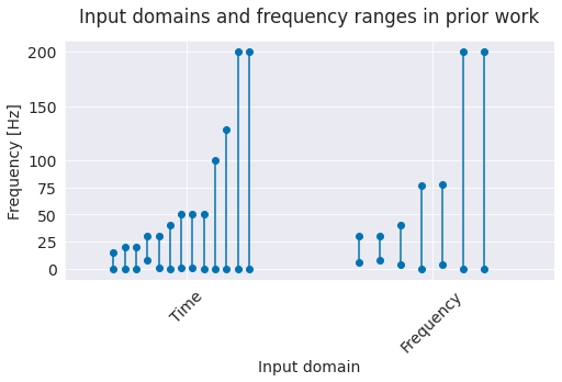
Fig. 1 Input domains and frequency ranges in prior work. Grey lines represent frequency ranges of individual studies. Note that many studies only include frequencies below 50 Hz, some use very restricted ranges (alpha/beta band).

Deep networks can either decode directly from the time-domain EEG or process the data in the frequency domain, for example after a Fourier transformation. 12 of the prior studies used time-domain inputs, 6 used frequency-domain inputs and one used both. We decided to work directly in the time domain, as the deep networks should in principle be able to learn how to extract any needed spectral information from the time-domain input.

Most prior studies that were working in the time domain only used frequencies below 50 Hz. We were interested in how well deep networks can also extract lesser-used higher-frequency components of the EEG signal. For that, we used a sampling rate of 250 Hz, which means we were able to analyze frequencies up to the Nyquist frequency of 125 Hz. As a suitable dataset where high-frequency information may help decoding, we included our high-gamma dataset in our study, since it was recorded specifically to allow extraction of higher-frequency (>50 Hz) information from scalp EEG [Schirrmeister et al., 2017].

Network Architectures

Show code cell source Hide code cell source

ls = np.array([' 2/2 ', ' 3/1 ', ' 2/2 ', ' 3/2 ', ' 1/1 ', ' 1/2 ', ' 1/3 ',
       ' 1–2/2 ', ' 3/1 (+ LSTM as postprocessor) ', ' 4/3 ', ' 1-3/1-3 ',
       ' 3–7/2 (+ LSTM or other temporal post-processing (see design choices)) ',
       ' 2/1 ', ' 3/3 (Spatio-temporal regularization) ',
       ' 2/2 (Final fully connected layer uses concatenated output by convolutionaland fully connected layers) ',
       ' 1-2/1 ',
       '2/0 (Convolutional deep belief network, separately trained RBF-SVM classifier) ',
       ' 3/1 (Convolutional layers trained as convolutional stacked autoencoder with target prior) ',
       ' 2/2 '])

conv_ls = [l.split('/')[0] for l in ls]
low_conv_ls = [int(re.split(r'[–-]', c)[0])for c in conv_ls]
high_conv_ls = [int(re.split(r'[–-]', c)[-1])for c in conv_ls]
dense_ls = [l.split('/')[1] for l in ls]
low_dense_ls = [int(re.split(r'[–-]', c[:8])[0][:2])for c in dense_ls]
high_dense_ls = [int(re.split(r'[–-]', c[:8])[-1][:2])for c in dense_ls]

all_conv_ls = np.concatenate([np.arange(low_c, high_c+1) for low_c, high_c in zip(low_conv_ls, high_conv_ls)])
all_dense_ls = np.concatenate([np.arange(low_c, high_c+1) for low_c, high_c in zip(low_dense_ls, high_dense_ls)])
bincount_conv = np.bincount(all_conv_ls)
bincount_dense = np.bincount(all_dense_ls)
rng = np.random.RandomState(98349384)
color = seaborn.color_palette()[0]
fig = plt.figure(figsize=(8,4))
for low_c, high_c in zip(low_conv_ls, high_conv_ls):
    offset = rng.randn(1) * 0.1
    tried_cs = np.arange(low_c, high_c+1)
    plt.plot([offset,] * len(tried_cs), tried_cs, marker='o', alpha=0.5, color=color, ls=':')
    
for i_c, n_c in enumerate(bincount_conv):
    plt.scatter(0.4, i_c, color=color, s=n_c*40)
    plt.text(0.535, i_c, str(n_c)+ "x", ha='left', va='center')

for low_c, high_c in zip(low_dense_ls, high_dense_ls):
    offset = 1 + rng.randn(1) * 0.1
    tried_cs = np.arange(low_c, high_c+1)
    plt.plot([offset,] * len(tried_cs), tried_cs, marker='o', alpha=0.5, color=color, ls=':')
    
for i_c, n_c in enumerate(bincount_dense):
    plt.scatter(1.4, i_c, color=color, s=n_c*40)
    plt.text(1.535, i_c, str(n_c)+ "x", ha='left', va='center')

plt.xlim(-0.5,2)
plt.xlabel("Type of layer")
plt.ylabel("Number of layers")
plt.xticks([0,1], ["Convolutional", "Dense"], rotation=45)
plt.yticks([1,2,3,4,5,6,7]);
plt.title("Number of layers in prior works' architectures", y=1.05)
glue('layernum_fig', fig)
plt.close(fig)
None

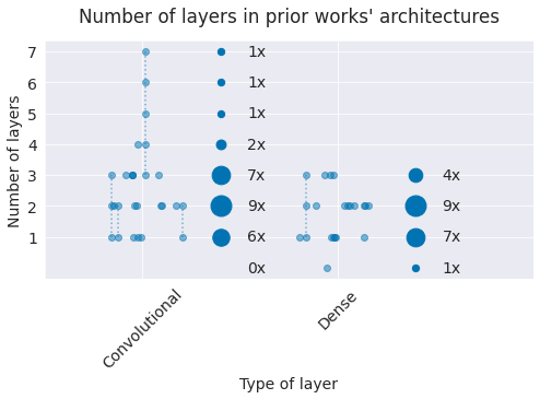
Fig. 2 Number of layers in prior work. Small grey markers represent individual architectures. Dashed lines indicate different number of layers investigated in a single study (e.g., a single study investigated 3-7 convolutional layers). Larger grey markers indicate sum of occurences of that layer number over all studies (e.g., 9 architectures used 2 convolutional layers). Note most architectures use only 1-3 convolutional layers.

The architectures used in prior work typically only included up to 3 layers, with only 2 studies considering more layers. As network architectures in other domains tend to be a lot deeper, we also evaluated architectures with a larger number of layers in our work. Several architectures from prior work also included fully-connected layers with larger number of parameters which had fallen out of favor in computer-vision deep-learning architectures due to their large compute and memory requirements with little accuracy benefit. Our architectures do not include traditional fully-connected layers with a large number of parameters.

Hyperparameter Evaluations

Table 2 Design choices and training strategies that prior deep-learning EEG decoding studies had studies.

Study	Design choices	Training strategies
[Lawhern et al., 2016]	Kernel sizes
[Sun et al., 2016]		Different time windows
[Tabar and Halici, 2017]	Addition of six-layer stacked autoencoder on ConvNet features Kernel sizes
[Liang et al., 2016]		Different subdivisions of frequency range Different lengths of time crops Transfer learning with auxiliary non-epilepsy datasets
[Hajinoroozi et al., 2016]	Replacement of convolutional layers by restricted Boltzmann machines with slightly varied network architecture}
[Antoniades et al., 2016]	1 or 2 convolutional layers
[Page et al., 2016]		Cross-subject supervised training, within-subject finetuning of fully connected layers
[Bashivan et al., 2016]	Number of convolutional layers Temporal processing of ConvNet output by max pooling, temporal convolution, LSTM or temporal convolution + LSTM
[Stober, 2016]	Kernel sizes	Pretraining first layer as convolutional autoencoder with different constraints
[Sakhavi et al., 2015]	Combination ConvNet and MLP (trained on different features) vs. only ConvNet vs. only MLP
[Stober et al., 2014]	Best values from automatic hyperparameter optimization: frequency cutoff, one vs two layers, kernel sizes, number of channels, pooling width	Best values from automatic hyperparameter optimization: learning rate, learning rate decay, momentum, final momentum
[Wang et al., 2013]	Partially supervised CSA
[Cecotti and Graser, 2011]	Electrode subset (fixed or automatically determined) Using only one spatial filter Different ensembling strategies

Prior work varied widely in their comparison of design choices and training strategies. 6 of the studies did not compare any design choices or training strategy hyperparameters. The other 13 studies evaluated different hyperparameters, with the most common one the kernel size (see Table 2). Only one study evaluated a wider range of hyperparameters [Stober et al., 2014]. To fill this gap, we compared a wider range of design choices and training strategies and specifically evaluated whether improvements of computer vision architecture design choices and training strategies also lead to improvements in EEG decoding.

Visualizations

Table 3 Visualizations presented in prior work.

Study	Visualization type(s)	Visualization findings
[Sun et al., 2016]	Weights (spatial)	Largest weights found over prefrontal and temporal cortex
[Manor et al., 2016]	Weights Activations Saliency maps by gradient	Weights showed typical P300 distribution Activations were high at plausible times (300-500ms) Saliency maps showed plausible spatio-temporal plots
[Tabar and Halici, 2017]	Weights (spatial + frequential)	Some weights represented difference of values of two electrodes on different sides of head
[Liang et al., 2016]	Weights Clustering of weights	Clusters of weights showed typical frequency band subdivision (delta, theta, alpha, beta, gamma)
[Antoniades et al., 2016]	Weights Correlation weights and interictal epileptic discharges (IED) Activations	Weights increasingly correlated with IED waveforms with increasing number of training iterations Second layer captured more complex and well-defined epileptic shapes than first layer IEDs led to highly synchronized activations for neighbouring electrodes
[Thodoroff et al., 2016]	Input occlusion and effect on prediction accuracy	Allowed to locate areas critical for seizure
[Shamwell et al., 2016]	Weights (spatial)	Some filter weights had expected topographic distributions for P300 Others filters had large weights on areas not traditionally associated with P300
[Bashivan et al., 2016]	Inputs that maximally activate given filter Activations of these inputs ”Deconvolution” for these inputs	Different filters were sensitive to different frequency bands Later layers had more spatially localized activations Learned features had noticeable links to well-known electrophysiological markers of cognitive load
[Stober, 2016]	Weights (spatial+3 timesteps, pretrained as autoencoder)	Different constraints led to different weights, one type of constraints could enforce weights that are similar across subjects; other type of constraints led to weights that have similar spatial topographies under different architectural configurations and preprocessings
[Manor and Geva, 2015]	Weights Mean and single-trial activations	Spatiotemporal regularization led to softer peaks in weights Spatial weights showed typical P300 distribution Activations mostly had peaks at typical times (300-400ms)
[Cecotti and Graser, 2011]	Weights	Spatial filters were similar for different architectures Spatial filters were different (more focal, more diffuse) for different subjects

Visualizations can help understand what information the networks are extracting from the EEG signal. 11 of the prior 19 studies presented any visualizations. These studies mostly focused on analyzing weights and activations, see Table 3. In our work, we first focused on investigating how far the networks extract spectral features known to work well for movement-related decoding, see Perturbation Visualization. Later, we also developed more sophisticated visualization methods and applied them both to pathology decoding, see Invertible Networks and Understanding Pathology Decoding With Invertible Networks.

Open Questions

• How do ConvNets perform on well-researched EEG movement-related decoding tasks against strong feature-based baselines?

• How do shallower and deeper architectures compare?

• How do design choices and training strategies affect the decoding performance?

• What features do the deep networks learn on the EEG signals?

• Do they learn to use higher-frequency (>50 Hz) information?