Generalization to Other Tasks#
Our architectures generalize well to a wide variety of decoding tasks
Perform similar or better than common feature-based algorithms on mental imageries, error decoding, auditory evoked potentials
Also perform well on intracranial EEG
Deep networks performs a bit better than shallow network on average across tasks
EEGNet architecture developed by others also performs well
Networks can be used in an online BCI scenario
After our initial work designing and evaluating convolutional neural networks for movement decoding from EEG, we evaluated the resulting networks on a wide variety of other EEG decoding tasks found that they generalize well to a large number of settings such as error-related decoding, online BCI control or auditory evoked potentials and also work on intracranial EEG. Text and content condensed from a number of publications, namely Schirrmeister et al. [2017], Völker et al. [2018], Burget et al. [2017], Volker et al. [2018], Behncke et al. [2018], Wang et al. [2018] and Heilmeyer et al. [2018]. In all of these works except Schirrmeister et al. [2017], I was not the main contributor, I assisted in adapting the code and training for the various settings and helped in the writing process.
Decoding Different Mental Imageries#
FBCSP |
Deep ConvNet |
Shallow ConvNet |
|---|---|---|
71.2 |
+1.0 |
-3.5 |
The Mixed Imagery Dataset (MID) was obtained from 4 healthy subjects (3 female, all right-handed, age 26.75±5.9 (mean±std)) with a varying number of trials (S1: 675, S2: 2172, S3: 698, S4: 464) of imagined movements (right hand and feet), mental rotation and mental word generation. All details were the same as for the High Gamma Dataset, except: a 64-electrode subset of electrodes was used for recording, recordings were not performed in the electromagnetically shielded cabin, thus possibly better approximating conditions of real-world BCI usage, and trials varied in duration between 1 to 7 seconds. The dataset was analyzed by cutting out time windows of 2 seconds with 1.5 second overlap from all trials longer than 2 seconds (S1: 6074 windows, S2: 21339, S3: 6197, S4: 4220), and both methods were evaluated using the accuracy of the predictions for all the 2-second windows for the last two runs of roughly 130 trials (S1: 129, S2: 160, S3: 124, S4: 123).
For the mixed imagery dataset, we find the deep ConvNet to perform slightly better and the shallow ConvNet to perform slightly worse than the FBCSP algorithm, as can be seen in Table 11.
Decoding Error-Related Signals#
Decoding Observation of Robots Making Errors#
robot task |
time interval |
Deep ConvNet |
rLDA |
FBCSP |
|---|---|---|---|---|
Pouring Liquid |
2-5s |
78.2 ± 8.4 |
67.5 ± 8.5 |
60.1 ± 3.7 |
Pouring Liquid |
3.3-7.5s |
71.9 ± 7.6 |
63.0 ± 9.3 |
66.5 ± 5.7 |
Lifting Ball |
4.8-6.3s |
59.6 ± 6.4 |
58.1 ± 6.6 |
52.4 ± 2.8 |
Lifting Ball |
4-7s |
64.6 ± 6.1 |
58.5 ± 8.2 |
53.1 ± 2.5 |
In this study, we aimed to classify whether a person had watched a video of a successful or an unsuccessful attempt of a robot performing one of two tasks (lifting a ball or pouring liquid) based on EEG recorded during the video observation. We compared the performance of our deep ConvNet to that of regularized linear discriminant analysis (rLDA) and FBCSP on this task. Our results, presented in Table 12, demonstrate that the deep ConvNet outperformed the other methods for both tasks and both decoding intervals.
Decoding of Eriksen Flanker Task Errors and Errors during Online GUI Control#
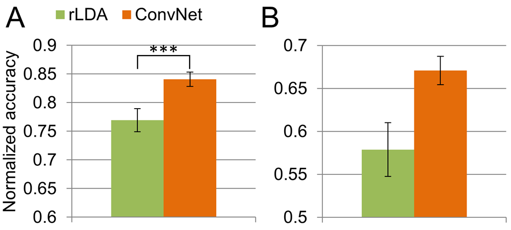
Fig. 31 Comparison of within-subject decoding by rLDA and deep ConvNets. Error bars show the SEM. A) Eriksen flanker task (mean of 31 subjects), last 20% of subject data as test set. Deep ConvNets were 7.12% better than rLDA, pval = 6.24 *10-20 (paired t-test). B) Online GUI control (mean of 4 subjects), last session of each subject as test data. Figure from [Völker et al., 2018]:#

Fig. 32 Mean normalized decoding accuracy on unknown subjects. Error bars show the SEM. A) Eriksen flanker task, trained on 30 subjects, tested on 1 subject. Deep ConvNets were 5.05% better than rLDA, p = 3.16 *10-4 (paired t-test). B) Online GUI control. Trained on 3 subjects, tested on the respective remaining subject. Figure from Völker et al. [2018].#
In two additional error-related decoding experiments, we evaluated an Eriksen flanker task and errors during an the online control of a graphical user interface through a brain-computer-interface. In the Eriksen flanker task, the subjects were asked to press the left or right button on a gamepad depending on whether an ‘L’ or an ‘R’ was the middle character of a 5-letter string displayed on the screen. For the online graphical user interface (GUI) control, the subjects were given an aim to reach using the GUI, also see Proof-of-Concept Assistive System. They had to think of one of the classes of the aforementioned Mixed Imagery Dataset to choose one of four possible GUI actions. The correct GUI action was always determined by the specificed aim given to the subject, hence an erroneous action could be detected. The decoding task in this paper was to distinguish whether the BCI-selected action was correct or erroneous. Results in Fig. 31 and Fig. 32 show that deep ConvNets outperform rLDA in all settings except cross-subject error-decoding for online GUI control, where the low number of subjects (4) may prevent the ConvNets to learn enough to outperform rLDA.
Proof-of-Concept Assistive System#
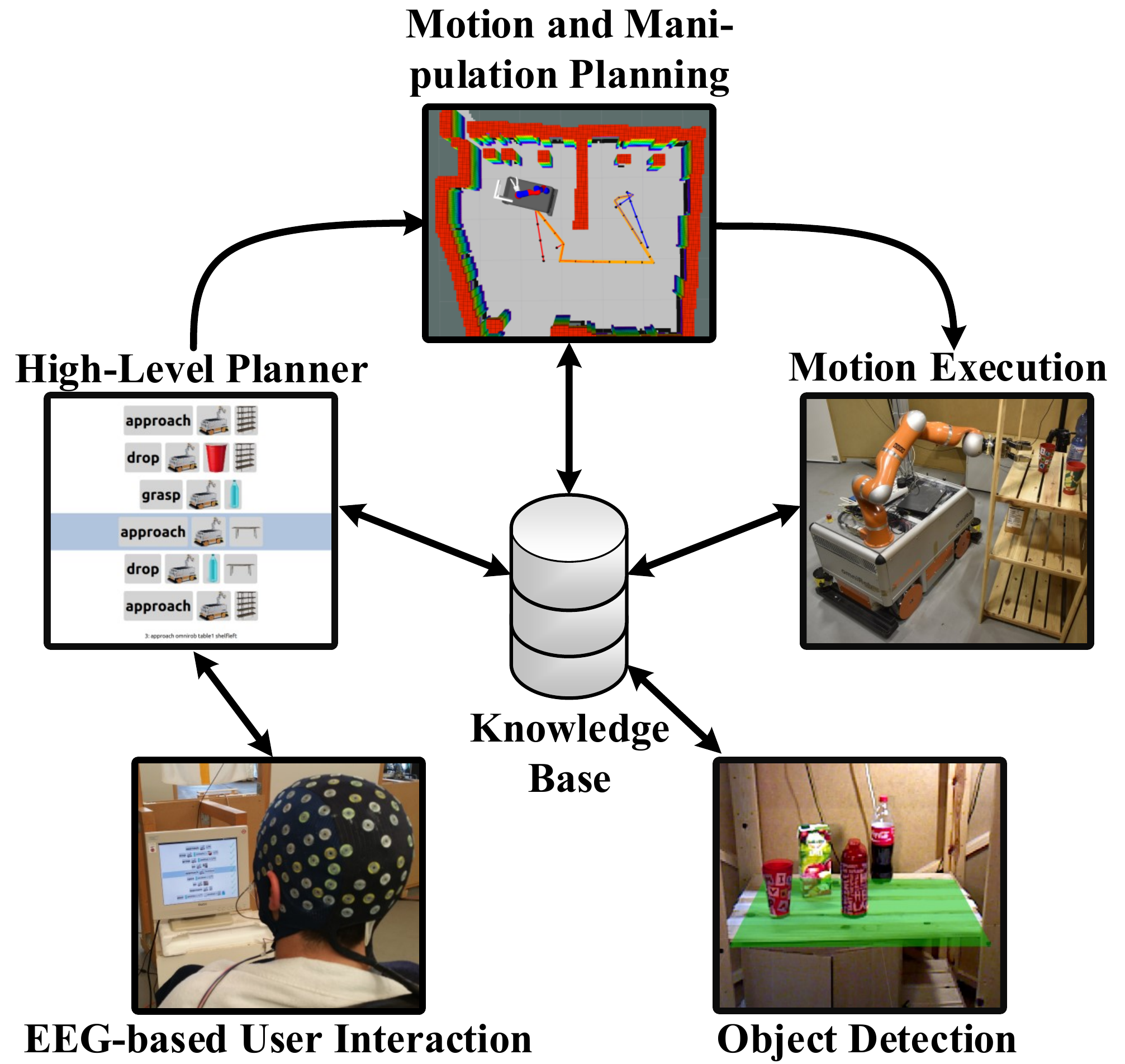
Fig. 33 Overview of the proof-of-concept assistive system from [Burget et al., 2017] using the deep ConvNet in the BCI component. Robotic arm could be given high-level commands via the BCI, high-level commands were extracted from a knowledge base. The commands were then autonomously planned and executed by the robotic arm. Figure from Burget et al. [2017]#
Subject |
Runs |
Accuracy* [%] |
Time [s] |
Steps |
Path Optimality [%] |
Time/Step [s] |
|---|---|---|---|---|---|---|
S1 |
18 |
84.1 ± 6.1 |
125 ± 84 |
13.0 ± 7.8 |
70.1 ± 22.3 |
9 ± 2 |
S2 |
14 |
76.8 ± 14.1 |
150 ± 32 |
10.1 ± 2.8 |
91.3 ± 12.0 |
9 ± 3 |
S3 |
17 |
82.0 ± 7.4 |
200 ± 159 |
17.6 ± 11.4 |
65.7 ± 28.9 |
11 ± 4 |
S4 |
3 |
63.8 ± 15.6 |
176 ± 102 |
26.3 ± 11.2 |
34.5 ± 1.2 |
6 ± 2 |
Average |
13 |
76.7 ± 9.1 |
148 ± 50 |
16.7 ± 7.1 |
65.4 ± 23.4 |
9 ± 2 |
We also evaluated the use of our deep ConvNet as part of an assistive robot system where the brain-computer interface was sending high-level commands to a robotic arm. In this proof-of-concept system, the robotic arm could be instructed by the user via the BCI to fetch a cup and directly move the cup to the persons mouth to drink from it. An overview can be seen in Fig. 33. Results from Table 13 show that 3 out of 4 subjects had a command accuracy of more than 75% and were able to reach the target using less than twice the steps of the minimal path through the GUI (path optimality > 50%).
Intracranial EEG Decoding#
Intracranial EEG Decoding of Eriksen Flanker Task#
Classifier |
Balanced Accuracy [%] |
Accuracy Correct Class [%] |
Accuracy Error Class [%] |
|---|---|---|---|
Deep4Net |
59.28 ± 0.50 |
69.37 ± 0.44 |
49.19 ± 0.56 |
ShallowNet |
58.42 ± 0.32 |
74.83 ± 0.25 |
42.01 ± 0.40 |
EEGNet |
57.73 ± 0.52 |
57.78 ± 0.48 |
57.68 ± 0.56 |
rLDA |
53.76 ± 0.32 |
76.12 ± 0.26 |
31.40 ± 0.38 |
ResNet |
52.45 ± 0.21 |
95.47 ± 0.14 |
09.43 ± 0.28 |
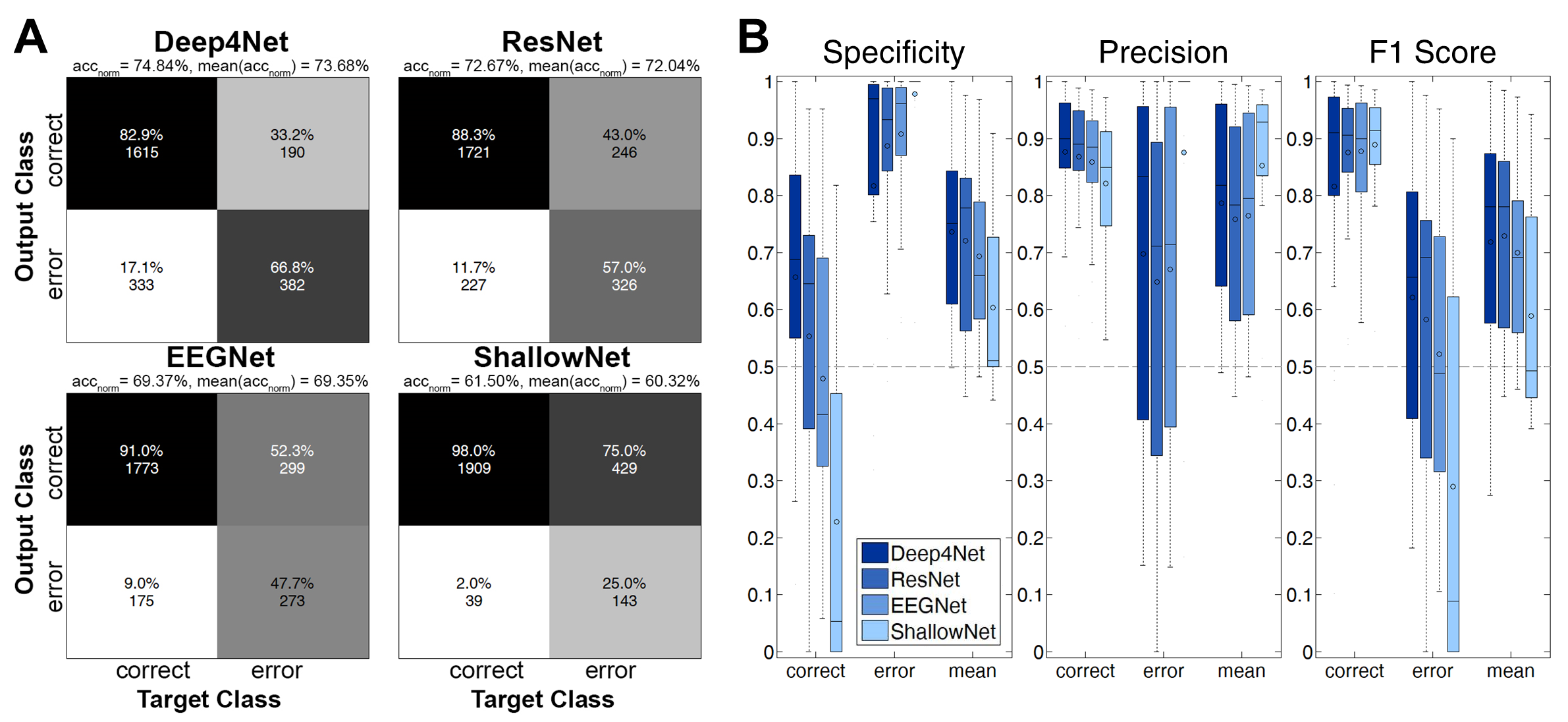
Fig. 34 Results for all-channel intracranial decoding of errors during an Eriksen flanker task. Here, the classifiers were trained on all available channels per patient. A) Confusion matrices of the four models used for decoding. The matrices display the sum of all trials over the 24 recordings. On top of the matrices, the class-normalized accuracy (average over per-class accuracies) over all trials, i.e., \(\mathrm{acc}_\mathrm{norm}\), and the mean of the single recordings’ normalized accuracy, i.e., \(\mathrm{mean}(\mathrm{acc}_\mathrm{norm})\) is displayed; please note that these two measures differ slightly, as the patients had a varying number of total trials and trials per class. B) Box plots for specificity, precision and F1 score. The box represents the interquartile range (IQR) of the data, the circle within the mean, the horizontal line depicts the median. The lower whiskers include all data points that have the minimal value of \(25^\mathrm{th} \mathrm{percentile}-1.5 \cdot \mathrm{IQR}\), the upper whiskers include all points that are maximally \(75^\mathrm{th} \mathrm{percentile}+1.5 \cdot \mathrm{IQR}\). Figure from Volker et al. [2018].#
We further evaluated whether the same networks developed for noninvasive EEG decoding can successfully learn to decode intracranial EEG. Therefore, in one work we used the same Eriksen flanker task as described in Decoding of Eriksen Flanker Task Errors and Errors during Online GUI Control, but recorded intracranial EEG from 23 patients who had pharmacoresistant epilepsy [Volker et al., 2018]. Results for single-channel decoding Table 14 show the deep and shallow ConvNet to clearly outperform rLDA (59.3%/58.4% vs. 53.8%) , whereas the residual ConvNet has low accuracy (52.5%). In contrast, results for all-channel decoding Fig. 34 show the residual ConvNet to perform well with the residual ConvNet and the deep ConvNet outperforming the shallow ConvNet (72.1% and 73.7% vs. 60.3% class-normalized accuracies (average over per-class accuracies)).
Transfer Learning for Intracranial Error Decoding#
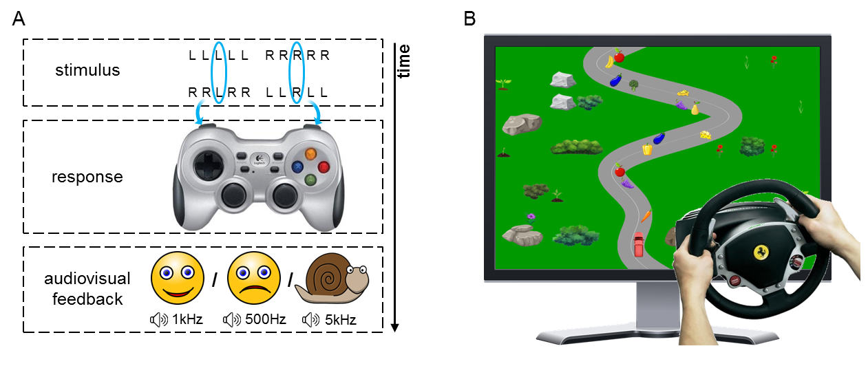
Fig. 35 Sketch of the Eriksen flanker task (A) and screenshot of the car driving task (B). Figure from Behncke et al. [2018].#
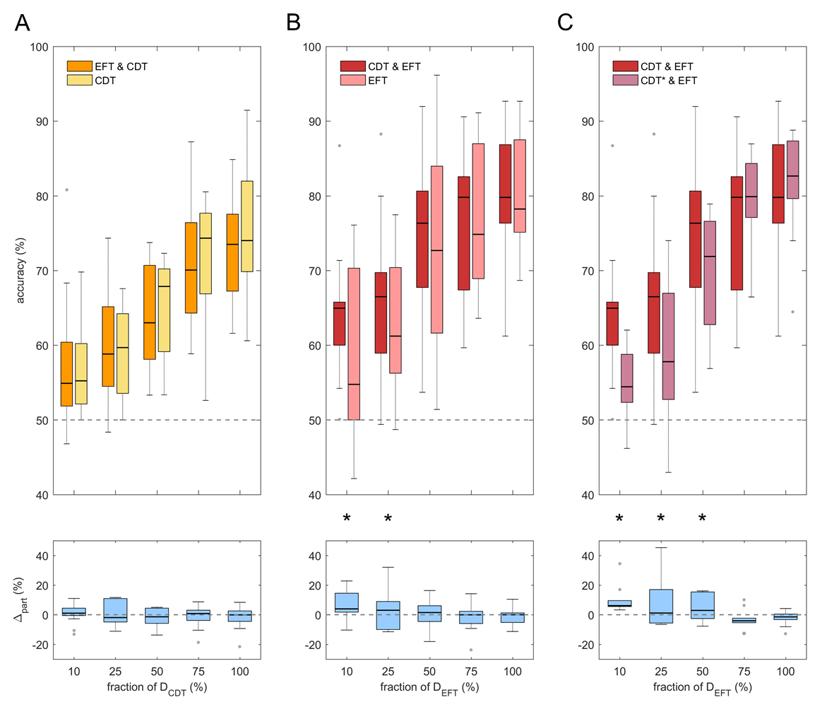
Fig. 36 Results for transfer learning on the Eriksen flanker task (EFT) and the car driving task (CDT). All results are computed for a varying fraction of available data for the target decoding task (bottom row). A compares CDT accuracies after training only on CDT or pretraining on EFT and finetuning on CDT. B compares EFT accuracies after only training on EFT or after pretraining on CDT and finetuning on EFT. As a sanity check for the results in B, C compares EFT accuracies when pretraining on original CDT data and finetuning on EFT to pretraining on CDT data with shuffled labels (CDT*) and finetuning on EFT. Results show that pretraining on CDT helps EFT decoding when little EFT data is available. Figure from Behncke et al. [2018].#
We further tested the potential of ConvNets to transfer knowledge learned from decoding intracranial signals in error-decoding paradigm to decoding signals in another a different error-decoding paradigm [Behncke et al., 2018]. The two error-decoding paradigms were the aforementioned Eriksen flanker task (EFT) and a car driving task (CDT), where subjects had to use a steering wheel to steer a car in a computer game and avoid hitting obstacles, where hitting an obstacle was considered an error event (see Fig. 35). Results in Fig. 36 show that pretraining on CDT helps EFT decoding when few EDT data is available.
Microelectrocorticography Decoding of Auditory Evoked Responses in Sheep#
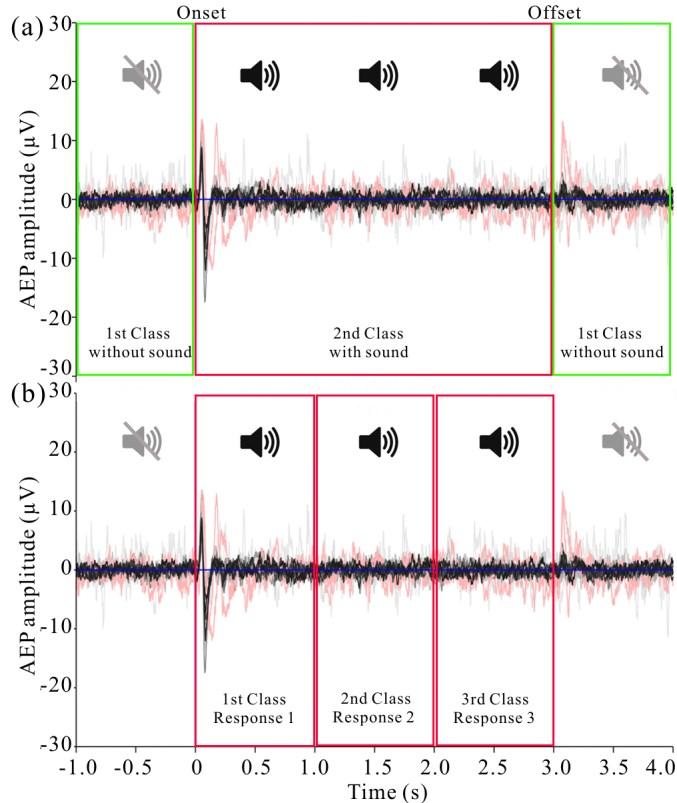
Fig. 37 [Behncke et al., 2018].Overview over decoding tasks for auditory evoked responses in a sheep.** First task (top) was to distingish 3 seconds when the sound was playing from the second before and the second after. Second task (bottom) was to distinguish the first, second and third second during theplaying of the sound. Signals are averaged responses from one electrode during different days, with black and grey being signals while the sheep was awake and red ones while the sheep was under general anesthesia. Figure from Wang et al. [2018].#
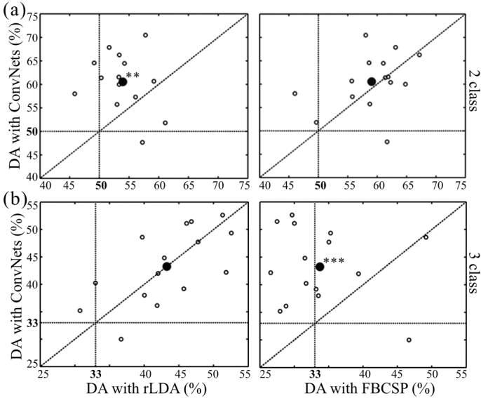
Fig. 38 Results of decoding auditory evoked responses from sheep with rlDA and FBSCP or the deep ConvNet. Open circles represent accuracies for individual experiment days and closed circles represent the average over these accuracies. Figure from Wang et al. [2018].#
In this study, we evaluated the ConvNets for decoding auditory evoked responses played to a sheep that was chronically implanted with a μECoG-based neural interfacing device [Wang et al., 2018]. 3-seconds-long sounds were presented to the sheep and two decoding tasks were defined from those 3 seconds as well as the second immediately before and after the playing of the sound. The first decoding task was to distinguish the 3 seconds when the sound was playing from the second immediately before and the second immediately after the sound. The second task was distinguishing the first, second and third second of the playing of the sound to discriminate early, intermediate and late auditory evoked response (see Fig. 37). Results in Fig. 38 show that the deep ConvNet can perform as good as FBSCP and rLDA, and perform well on both tasks, whereas rLDA performs competitively only on the first and FBSCP only on the second task.
Evaluation on Large-Scale Task-Diverse Dataset#
Name (Acronym) |
#Classes |
Task Type |
#Subjects |
Trials per Subject |
Class balance |
|---|---|---|---|---|---|
High-Gamma Dataset (Motor) |
4 |
Motor task |
20 |
1000 |
balanced |
KUKA Pouring Observation (KPO) |
2 |
Error observation |
5 |
720-800 |
balanced |
Robot-Grasping Observation (RGO) |
2 |
Error observation |
12 |
720-800 |
balanced |
Error-Related Negativity (ERN) |
2 |
Eriksen flanker task |
31 |
1000 |
1/2 up to 1/15 |
Semantic Categories |
3 |
Speech imagery |
16 |
750 |
balanced |
Real vs. Pseudo Words |
2 |
Speech imagery |
16 |
1000 |
3/1 |
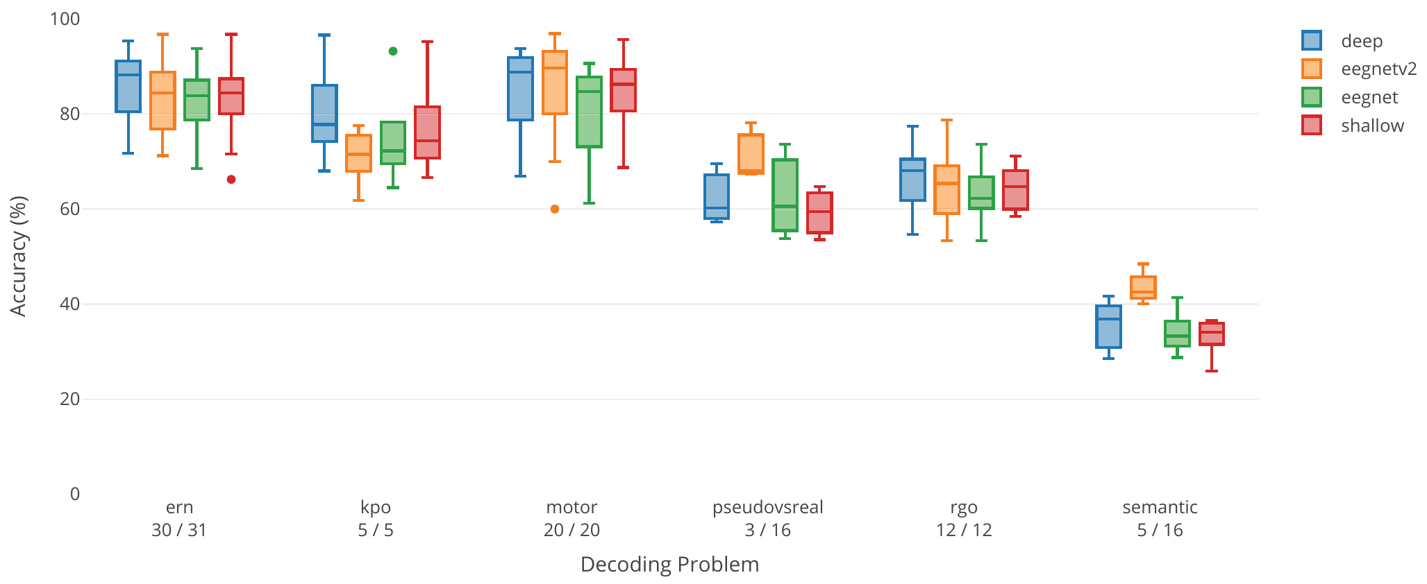
Fig. 39 Per-dataset results for the large-scale evaluation of deep ConvNet, shallow ConvNet and two versions of EEGNet. Boxplots show the distribution over per-subject accuracies for the individual decoding tasks. ern, kpo and rgo are the error-related datasets, ern: Error-related negativity Eriksen flanker task, KPO: KUKA Pouring Observation paradigm, rgo: robot-grasping observation paradigm. motor is the high-gamma dataset with 6 additional subjects that were excluded for data quality reasons from [Schirrmeister et al., 2017]. pseudovsreal and semantic are two semantic processing datasets to classify silent repetitions of pseudowords vs. realwords (pseudovsreal) or different semantic categories (semantic) . Figure from Heilmeyer et al. [2018].#
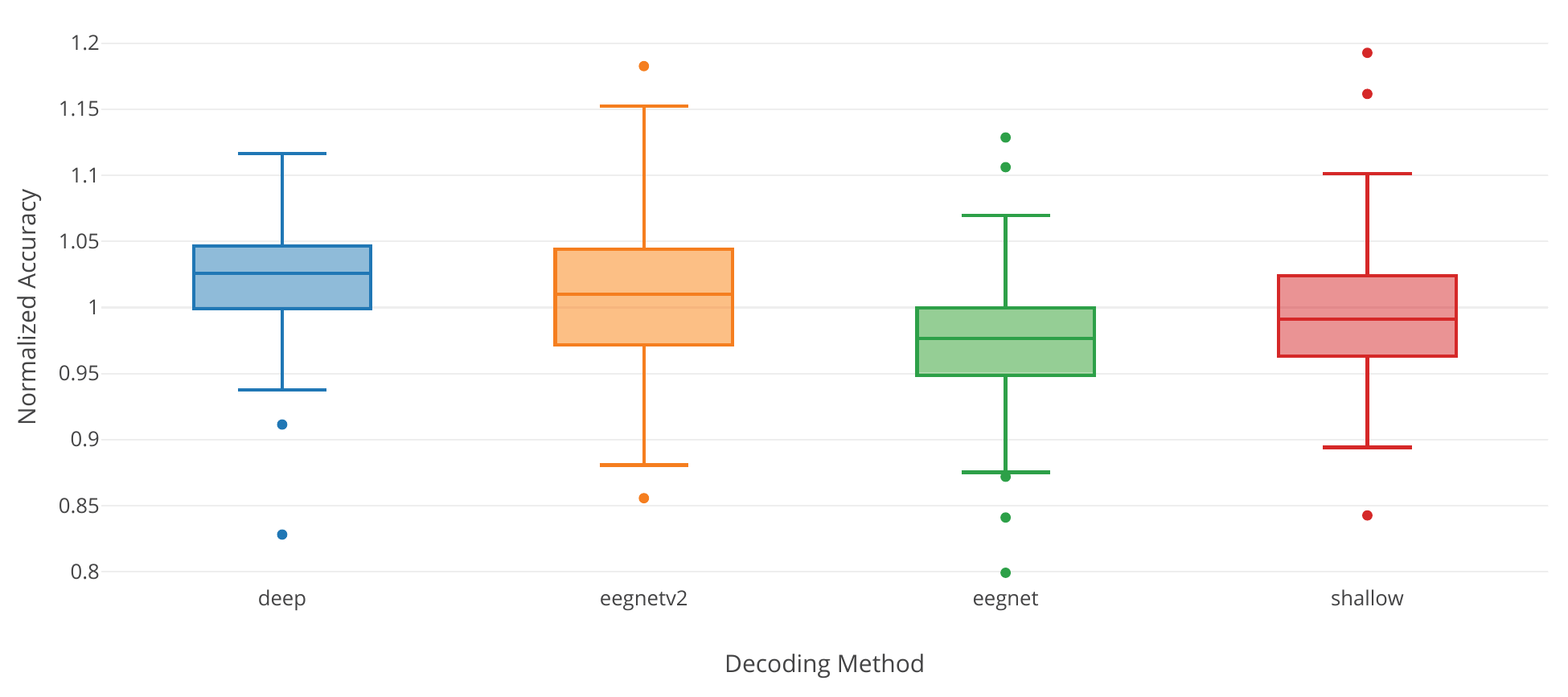
Fig. 40 Dataset-averaged results for the large-scale evaluation of deep ConvNet, shallow ConvNet and two versions of EEGNet. Accuracies are normalized to the average of the accuracies of all models. Figure from Heilmeyer et al. [2018].#
Mean accuracy |
Mean normalized accuracy |
|
|---|---|---|
Deep ConvNet |
70.08% ± 20.92% |
1.00 ± 0.05 |
EEGNetv2 |
70.00% ±18.86% |
1.02 ± 0.08 |
EEGNet |
67.71% ± 19.04% |
0.98 ± 0.06 |
Shallow ConvNet |
67.71% ±19.04% |
0.99 ± 0.06 |
We also compared the deep and shallow ConvNet architectures as well as EEGNet on six classification tasks with more than 90000 trials in total (see Table 15) [Heilmeyer et al., 2018]. The datasets tasks were all recorded in our lab and included the high-gamma dataset, three error-related tasks described before (Eriksen flanker task, robot grasping and robot pouring observations) as well as two tasks on semantic processing. In the semantic processing dataset, the classification tasks were to distinguish different types of words that a subject silently repeated [Rau, 2015]. The first task was to distinguish existing real words from nonexisting pseudowords. The second classification task was to distingiush three semantic categories (food, animals, tools) the word may belong to. The evaluation code for all models always used the original code and hyperparameters from the original studies in order to ensure a fair comparison. Results show that the deep ConvNet and the more recent version of EEGNet (EEGNetv2) perform similarly well, with shallow and an older version of EEGNet performing slightly worse, see Fig. 39, Fig. 40 and Table 16.
Open Questions
How do these networks perform on non-trial-based tasks like pathology decoding?