Perturbation Visualization#
Perturbation visualization perturbs spectral features and measures change in classification predictions
Can be used to investigate well-known spectral power features
Can also be implemented through gradients of spectral power features
Can be extended to investigate phase features
What features the EEG-decoding ConvNet learns is a scientifically interesting question and not straightforward to answer. Through end-to-end training, the networks may learn a variety of features, including brain-signal features and non-brain-signal features, e.g., eye movements that correlate to a hand movement. The learned features may be already known from prior research on brain-signal decoding or represent novel features that had not been described in the literature. However, there is no straightforward way to find out what the deep networks have learned from the brain signals.
Therefore, we developed an input amplitude perturbation method to investigate whether the deep networks learn to extract spectral amplitude features, which are very commonly used in many EEG decoding pipelines. For example, it is known that the amplitudes, for example of the alpha, beta and gamma bands, provide class-discriminative information for motor tasks [Ball et al., 2008, Pfurtscheller, 1981, Pfurtscheller and Aranibar, 1979]. Hence, it seems a priori very likely that the deep networks learn to extract such features and worthwhile to check whether they indeed do so. We also extended this method to investigate the use of phase information by the networks.
The amplitude perturbation method was developed by me in the context of this thesis, the phase perturbation method was developed by Kay Hartmann together with me. Text and figures in this chapter are adapted from [Schirrmeister et al., 2017] and [Hartmann et al., 2018].
Input-Perturbation Network-Prediction Correlation Map#
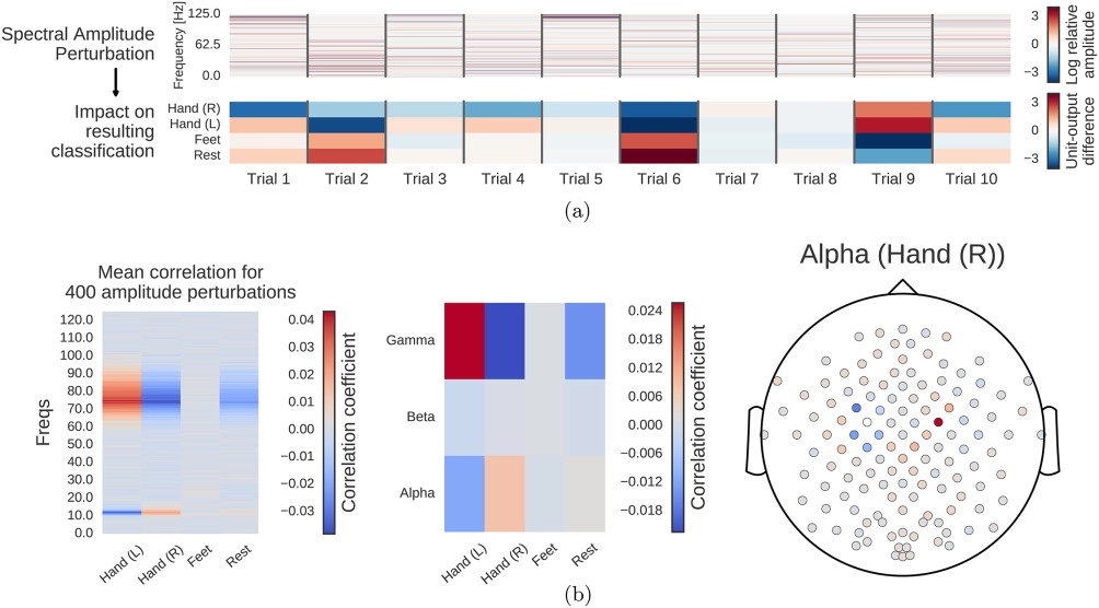
Fig. 12 Computation overview for input-perturbation network-prediction correlation map. (a) Example spectral amplitude perturbation and resulting classification difference. Top: Spectral amplitude perturbation as used to perturb the trials. Bottom: unit-output difference between unperturbed and perturbed trials for the classification layer units before the softmax. (b) Input-perturbation network-prediction correlations and corresponding network correlation scalp map for alpha band. Left: Correlation coefficients between spectral amplitude perturbations for all frequency bins and differences of the unit outputs for the four classes (differences between unperturbed and perturbed trials) for one electrode. Middle: Mean of the correlation coefficients over the the alpha (7–13 Hz), beta (13–31 Hz) and gamma (71–91 Hz) frequency ranges. Right: An exemplary scalp map for the alpha band, where the color of each dot encodes the correlation of amplitude changes at that electrode and the corresponding prediction changes of the ConvNet. Negative correlations on the left sensorimotor hand/arm areas show an amplitude decrease in these areas leads to a prediction increase for the Hand (R) class, whereas positive correlations on the right sensorimotor hand/arm areas show an amplitude decrease leads to a prediction decrease for the Hand (R) class. Figure from [Schirrmeister et al., 2017].#
To investigate the causal effect of changes in power on the deep ConvNet, we correlated changes in ConvNet predictions with changes in amplitudes by perturbing the original trial amplitudes (see Fig. 12 for an overview). Concretely, tbe visualization method performs the following steps:
Transform all training trials into the frequency domain by a Fourier transformation
Randomly perturb the amplitudes by adding Gaussian noise (with mean 0 and variance 1) to them (phases were kept unperturbed)
Retransform perturbed trials to the time domain by the inverse Fourier transformation
Compute predictions of the deep ConvNet for these trials before and after the perturbation (predictions here refers to outputs of the ConvNet directly before the softmax activation)
Repeat this procedure with 400 perturbations sampled from aforementioned Gaussian distribution
Correlate the change in input amplitudes (i.e., the perturbation/noise we added) with the change in the ConvNet predictions.
To ensure that the effects of our perturbations reflect the behavior of the ConvNet on realistic data, we also checked that the perturbed input does not cause the ConvNet to misclassify the trials (as can easily happen even from small perturbations, see [Szegedy et al., 2014]. For that, we computed accuracies on the perturbed trials. For all perturbations of the training sets of all subjects, accuracies stayed above 99.5% of the accuracies achieved with the unperturbed data.
This method can not only be applied to final predictions, but also to investigate any intermediate network filter’s activations in order to better understand the intermediate computations of the network.
Gradient-Based Implementation#
An simpler and more computationally efficient way to implement the idea of testing the sensitivity of the network to spectral amplitude features is through gradient-based analysis 1. There, we directly compute the gradient of the output unit with respect to the amplitudes of all frequency bins of all electrodes of the original unperturbed trial. To practically implement this, one must first transform the time domain input signal into the frequency domain and to a amplitude/phase representation via the Fourier transform. Then, one can transform the amplitude/phase representation back to the time domain using the inverse Fourier Transform. Since the inverse Fourier transform is differentiable, one can backpropagate the gradients from the output unit through the time domain input back to the amplitudes. The more the network behaves locally linear around the input, the closer the results of this variant would be to the original perturbation variant. It is computationally substantially faster as everything is computed in one forward-backward pass, without needing to iterate over many perturbations. The gradient-based method may result in less insightful visualizations if the prediction function of the network is locally very nonlinear at a given pint but has an approximately linear relationship with the spectral amplitudes in a larger neighbourhood around that point. See works on other saliency/gradient-based visualizations for discussions in this topic, e.g. Sturmfels et al. [2020].
Extension to Phase-Based Perturbations#
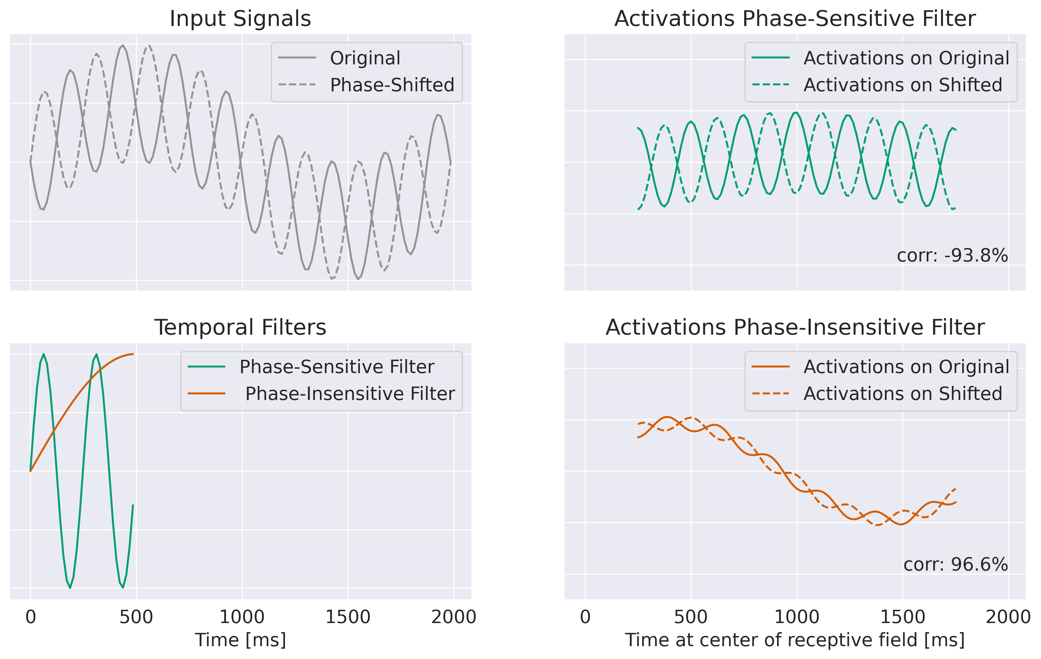
Fig. 13 Example showing the intution of the phase perturbation correlation method. Shown are top left: two input signals where the phase of one frequency has been shifted between the two signals; bottom left: two temporal filters, one phase-sensitive and one phase-insensitive to the frequency where the phase was shifted; right: activations for the phase-sensitive and phase-insensitive filter for the original and the shifted signal. Note that correlation between activations of the phase-sensitive filter is very low, even negative (-93.8%), whereas correlation between the activations of the phase-insensitive filter remains high at 96.6%. Note that this simplified example does not illustrate some key mechanisms for activations to become more generally phase-insensitive such as nonlinearities and pooling operations.#
The amplitude-perturbation method can also be extended to investigate in how far networks are affected by changes in phase features. The response of filters to changes in the phase of certain frequencies was calculated similarly to the amplitude perturbation correlations. However, because of the cyclic nature of phase features, the change of activations in a filter resulting from a phase shift cannot be quantified using the mean activation difference. When you change the phase of the frequency that a filter is sensitive to, you won’t expect the activations of the filter to increase uniformly throughout the window. Instead, the activations of a phase-sensitive filter will probably be temporally shifted by the phase change. Units of filters whose receptive field contained its specific phase in the original signal should activate less and units whose receptive field contains the specific phase in the perturbed signal should then activate more. Therefore, the original activations and the activations on the perturbed input should have a decreased correlation (less than 1). Activation and correlation should remain similar for phase-insensitive filters.
Phase perturbations were sampled from \(p^{P}_{\xi,i}{\sim}N(0,\pi)\). Perturbed phases \(P^{P}_\xi\) were calculated by shifting the phase: \(P^{P}_\xi(X_i)=p^{P}_{\xi,i}+P_\xi(X_i)\). Perturbed signals \(X^{P}\) were reconstructed by inverse Fourier transformation. The correlation between original and perturbation filter activations of a filter \(f\) from trial \(i\) is denoted by \(\rho_{y_{f,i},y^{P}_{f,i}}=corr(y_{f,i},y^{P}_{f,i})\). Correlations between phase perturbations \(p^{P}_{\xi}\) and filter activity correlations \(\rho_{y_{f},y^{P}_{f}}\) were calculated identically to amplitude perturbations. The resulting mean absolute phase perturbation correlations for each layer is denoted as \(\varrho^P_{l,\xi}\).
Since we wanted to study only the effect of changing the overall phase of the signal, independent of the effect of increased or decreased phase synchronicity across EEG channels, we did not perturb the phase in channels individually, but applied one phase perturbation of a certain frequency in all channels equally.
Interpretation and Limitations#
The perturbation-based visualization reflects network behavior and one cannot directly draw inferences about the data-generating process from it. This is because a prediction change caused by an amplitude perturbation may reflect both learned task-relevant factors as well as learned noise correlations. For example, increasing the alpha-band amplitude at electrode C4 (located on the right side), may increase the predicted probability for right hand movement. That would likely not be because the alpha amplitude actually increases at C4 during right hand movement, but because the amplitude decreases on C3 and is correlated between C3 and C4. Hence, first subtracting the C4 amplitude from the C3 amplitude and then decoding associating negative values of this computation with right hand movement is a reasonable learned prediction function. And this learned prediction function would cause the amplitude-perturbation function to show that an alpha increase at C4 causes an increase in the predicted probability for right hand movement. For a more detailed discussion of this effect in the context of linear models, see [Haufe et al., 2014].
Open Questions
Do spectral maps obtained from this visualization show neurophysiologically plausible patterns?
What can they reveal about the inner computations of the networks?
- 1
This idea was suggested to us in personal communication by Klaus-Robert Müller.