Understanding Pathology Decoding With Invertible Networks

EEG-InvNet and EEG-CosNet can reveal learned features for EEG pathology decoding

• EEG-InvNet can reach 85.5% accuracy, competitive with regular ConvNets

• Visualizations show networks learn well-known features like temporal slowing or occipital alpha

• Visualizations also reveal surprising learned features in the very low frequencies up to 0.5 Hz

After our initial work on pathology decoding, we wanted to gain a deeper understanding of the features deep networks learn to distinguish healthy from pathological recordings. For that, we used invertible networks as generative classifiers since they offer more ways to visualize their learned prediction function in input space. Our EEG-InvNet reached competitive accuracies on the pathology decoding task. We visualize prototypes of the two classes as well as individual electrode signals predictive of a certain class independent of the signals at other electrodes. These visualizations revealed both well-known features like temporal slowing or occipital alpha as well as surprising patterns in the very low frequencies (<= 0.5 Hz). To gain an even better understanding, we distilled the invertible network’s knowledge into a very small network called EEG-CosNet that is interpretable by design. These visualizations showed regular patterns in the alpha and beta range associated with healthy recordings and a diverse set of more irregular waveforms associated with pathology. For the very low frequencies, visualizations revealed a frontal component predicting the healthy class and other components with spatial topographies including the temporal areas predicting the pathological class.

All work presented in this chapter is novel unpublished work performed by me in the context of this thesis.

Dataset, Training Details and Decoding Performance

Table 20 Accuracy of Invertible Network in comparison with accuracies of regular ConvNets.

Deep	Shallow	TCN	EEGNet	EEG-InvNet
84.6	84.1	86.2	83.4	85.5

We apply our EEG-InvNet to pathology decoding on the same TUH dataset as in Decoding Pathology. We use only 2 minutes of each recording at 64 Hz, and input 2 seconds as one example to the invertible network. This reduced dataset allows fast experimentation while still yielding good decoding performance. We used AdamW [Loshchilov and Hutter, 2019] as our optimizer and cosine annealing with restarts [Loshchilov and Hutter, 2017] every 25 epochs as our learning rate schedule. We emphasize these details were not heavily optimized for maximum decoding performance, but rather chosen to obtain a robustly performing model worth investigating more deeply. Results in Table 20 show that our EEG-InvNet compares similar than regular ConvNets, even better than some ConvNets, therefore motivating a deeper investigation into its learned features.

Class Prototypes

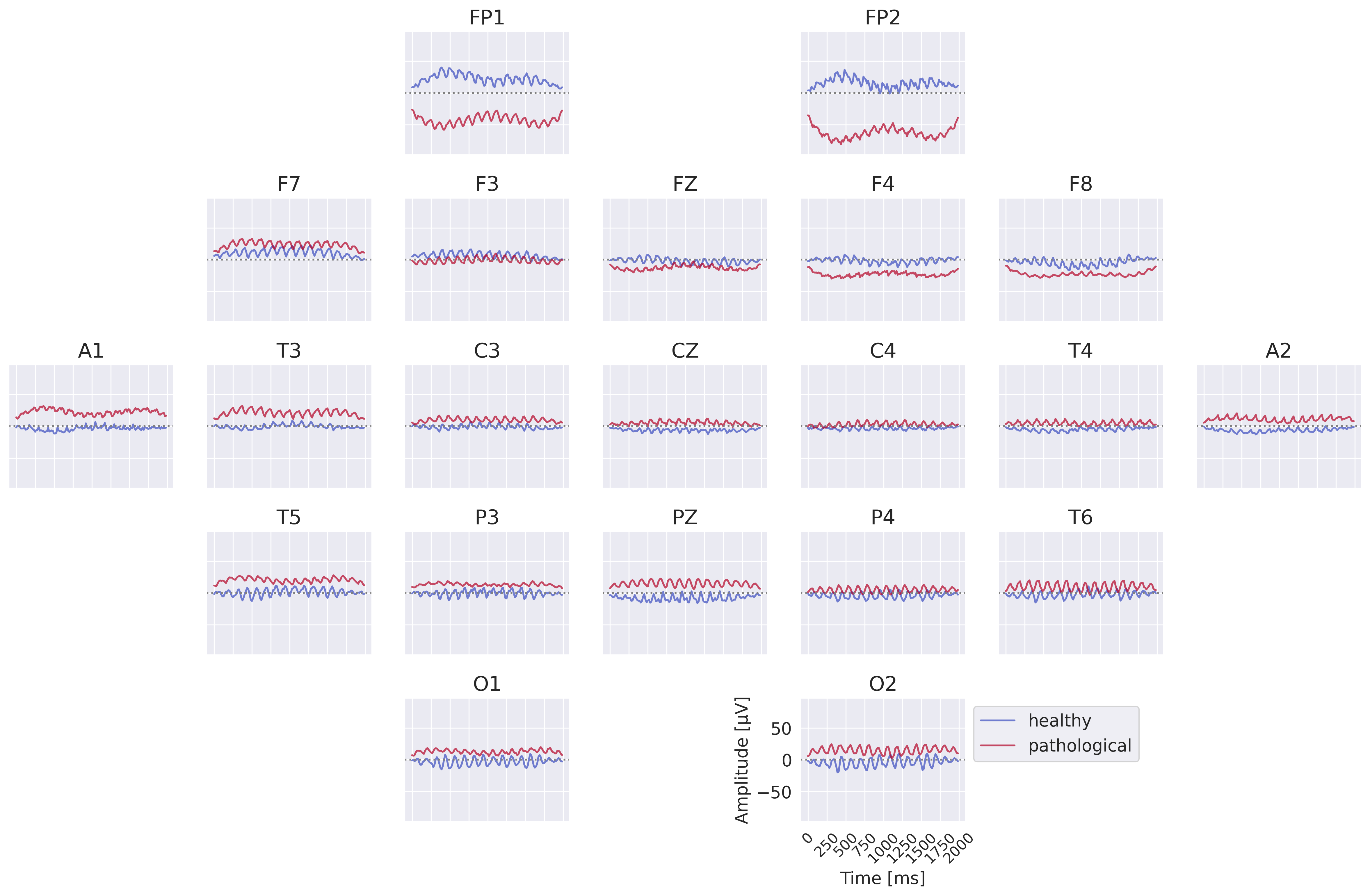
Fig. 47 Learned class prototypes from EEG-InvNet. Obtained by inverting learned means of class-conditional gaussian distributions from latent space to input space through the invertible network trained for pathology decoding.

Class prototypes reveal known oscillatory features and surprisingly hint at the use of very-low-frequency information by the invertible network. We inverted the learned latent means of the healthy and the pathological class distributions back to the input space to visualize the most likely healthy and most likely pathological examples under the learned distribution, see also Class Prototypes. Visualizations in Fig. 47 show differences in the alpha rhythm like a stronger alpha rhythm at O1 in the healthy example. We also see further differences with a variety of different oscillatory patterns present for both classes. Surprisingly, there are also differences in the very low frequencies like substantially different mean values for FP1 and FP2 for the two class prototypes, which we will further investigate later. One challenge of this visualization is that one has to look at each prototype as one complete example and cannot interpret signals at individiual electrodes independently. This is what we tackle in our next visualization.

Per-Channel Prototypes

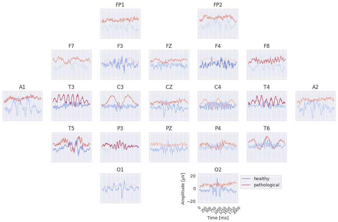
Fig. 48 Learned per-channel prototypes from EEG-InvNet. Each channels’ input is optimized independently to increase the invertible networks prediction for the respective class. During that optimization, signals for the other non-optimized channels are sampled from the training data. Color indicates average softmax prediction over 10000 samples for the other channels. Very prominent slowing patterns appear for the pathological class at mjultiple electrodes.

The per-channel prototypes reveal interesting learned features for the two classes (see Fig. 48). The pathological prototypes show strong low-frequency activity, for example at T3 and T4, consistent with slowing as a biomarker for pathology. The healthy signal shows alpha activity, for example at C4 and T6. Besides these patterns, a lot of other interesting patterns may be interesting to further investigate. One of them, the differences in the very low frequencies will be further explored below. Note that it was not possible to synthesize a signal that is clearly indicative of one class independent of the other electrodes for all electrodes. This is to be expected if the EEG-InvNet uses a feature inherently impossible to recreate within a single electrode like the degree of synchrony between signals at different electrodes.

EEG-CosNet Visualizations

Table 21 Accuracy of small interpretable network on invertible network predictions and original labels.

	EEG-InvNet Predictions	Original Labels
Train	92.5	89.1
Test	88.8	82.6

Fig. 49 Visualization of small interpretable EEG-CosNet trained to mimic the EEG-InvNet. Scalp Plots are spatial filter weights transformed to patterns, signals below each scalp plot show corresponding convolutional filter. Signal colors represent the weights of the linear classification layer, transformed to patterns (see EEG-CosNet for an explanation). Plots are sorted by these colors. Note that polarities of the scalp plots and temporal waveforms are arbitrary as absolute cosine similarities are computed on the spatially filtered and temporally convolved signals.

Results for the EEG-CosNet show that a large fraction of the predictions of the invertible network can be predicted from a relatively small number of mostly neurophysiologically plausible spatio-temporal patterns. EEG-CosNet predicts 88.8% of the recordings in the same way as the EEG-InvNet and retains a test set label accuracy of 82.6% (see Table 21. This shows that from just 64 spatiotemporal features, the EEG-CosNet is able to predict the vast majority of the EEG-InvNet predictions. Still, the remaining gap indicates that the EEG-InvNet has learned some features that the EEG-CosNet cannot represent.

Visualizations in Fig. 49 show more regular waveforms in the alpha and beta-frequency ranges with higher association for the healthy class and more waveforms in other frequency ranges as well as less regular waveforms with higher association for the pathological class. As examples for the healthy class, plots 1 and 3 show oscillations with a strong alpha component and plots 15-17 show oscillations with strong beta components. For the pathological class, we see slower oscillations, e.g., in plots 53 and 60, and also more irregular waveforms in, e.g., plots 49 and 52.

Investigation of Very Low Frequencies

One surprising observation from the visualizations are differences in the very low frequencies (<=0.5 Hz) between the two class prototypes. For example, the very different mean values in the class prototypes for FP1 and FP2 suggest very low frequency information differs between the two classes on those electrodes. These kinds of differences motivated us to more deeply investigate in how far very low frequency information is predictive of pathology.

Table 22 Accuracy on data lowpassed below 0.5 Hz.

EEG-InvNet	EEG-CosNet	Fourier-GMM
75.4	75.0	75.4

For this, we trained an EEG-InvNet on data lowpassed to be below 0.5 Hz. For the lowpass, we first removed all Fourier components above 0.5 Hz for each recording and also for each 2-second input window for the network. This retained 75.4% accuracy with the EEG-InvNet, indicating even these very low frequencies remain fairly informative about the pathologicality of the recording. We additionally trained the EEG-CosNet with a temporal filter spanning the entire input window length of 2 seconds and found it to retain 75% test accuracy. Finally, we also directly trained a 8-component gaussian mixture model Fourier-GMM in Fourier space. Only 3 dimensions per electrode remain: real value of the 0-Hz component ( summed values of the input window) and real and imaginary value of the 0.5-Hz Fourier component). Each of the 8 mixture components had learnable class weights, how much each mixture component contributed to that classes learned distribution. The Fourier-GMM also retains 75.4% test accuracy. All results are shown in Table 22.

EEG-InvNet Visualizations

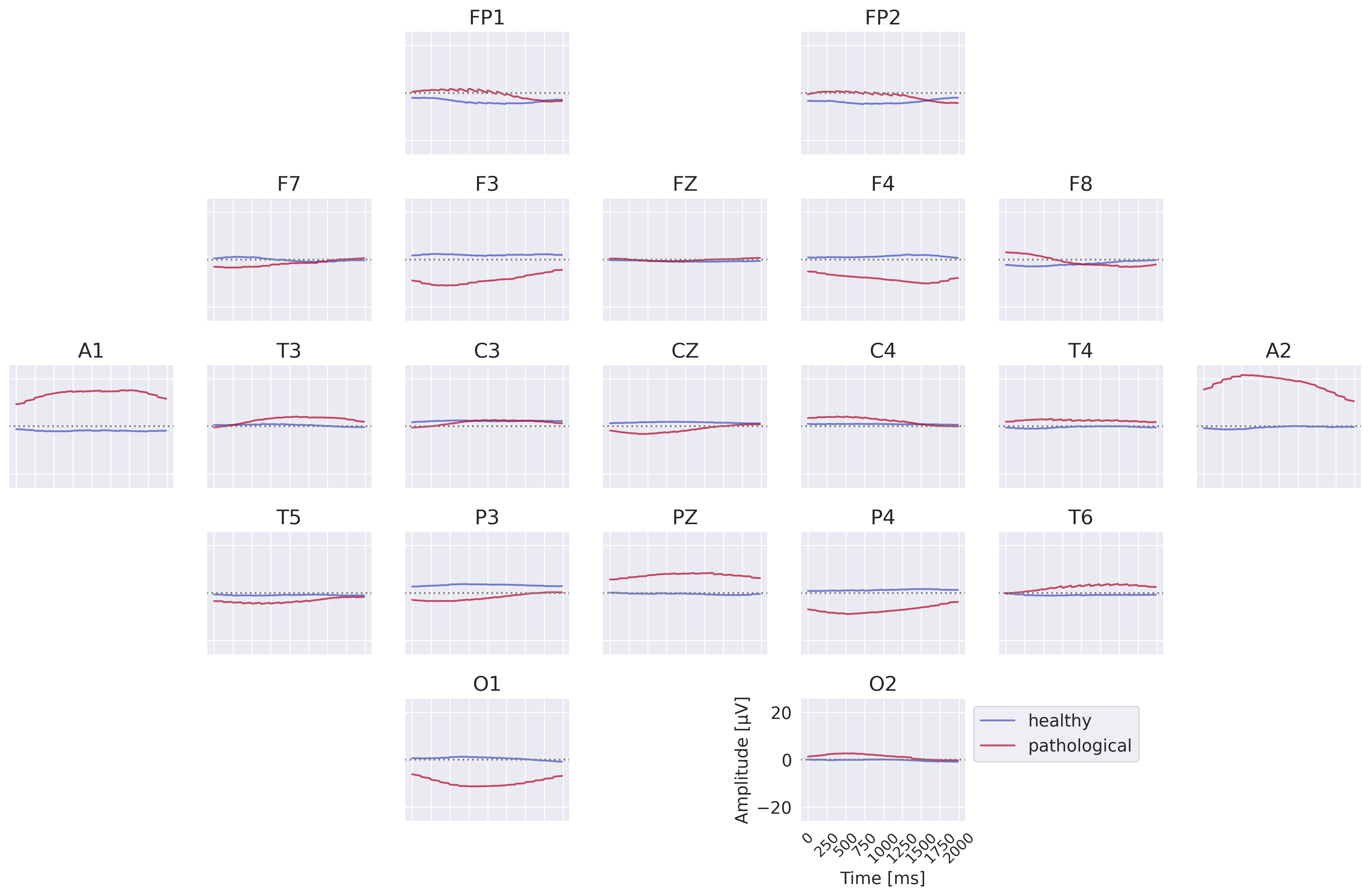
Fig. 50 Class prototypes for the EEG-InvNet trained on data lowpassed to be below 0.5 Hz. Note large differences at A1 and A2.

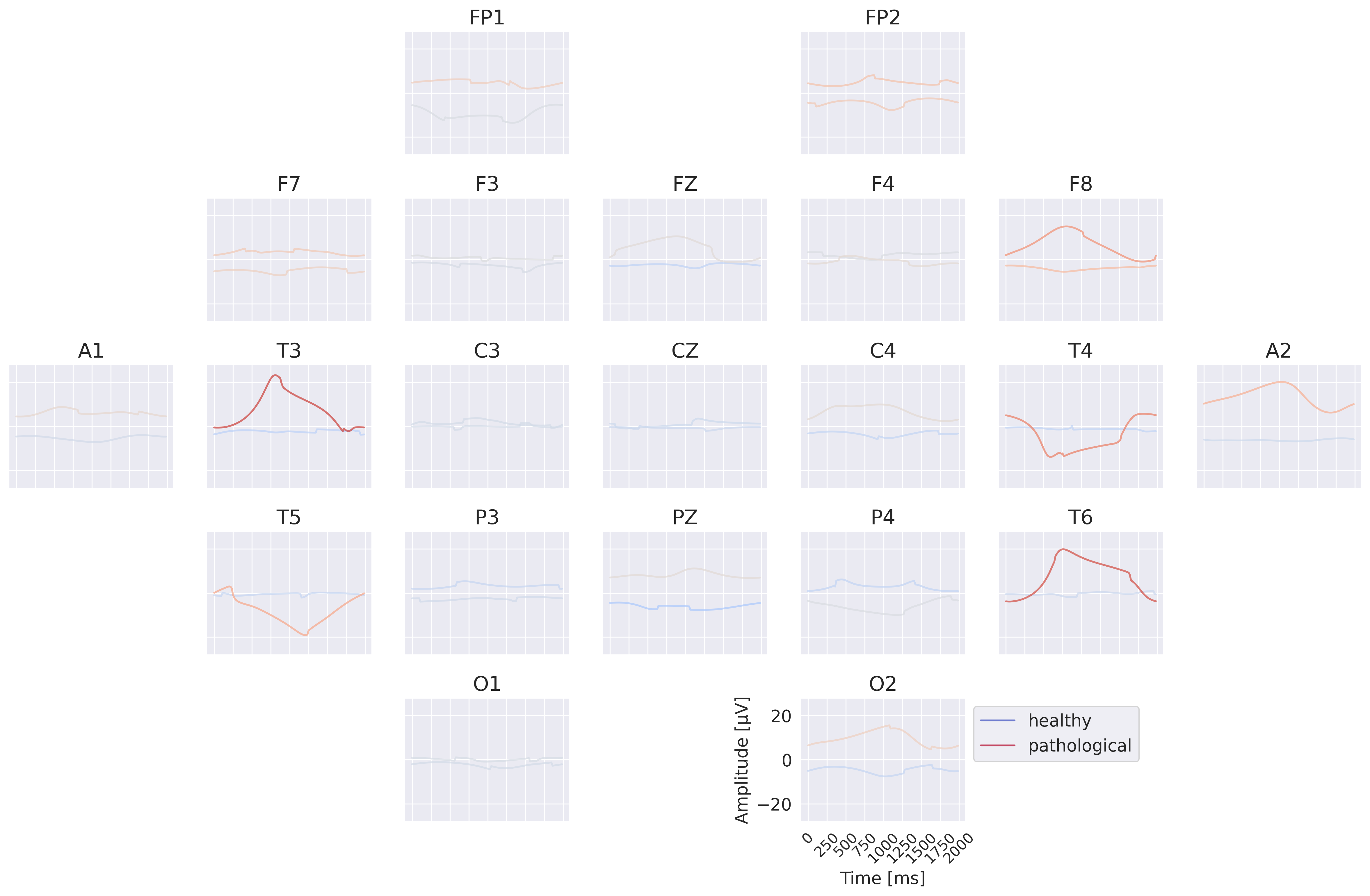
Fig. 51 Per-electrode prototypes for EEG-InvNet trained on data lowpassed below 0.5 Hz. Note strongly predictive signals at T3,T4,T6.

The visualizations of the EEG-InvNet show several interesting features. The class prototypes in Fig. 50 show differences at most electrodes, especially pronounced for A1 and A2. The per-electrode prototypes in Fig. 50 show predictive information in the T3,T4 and T6 electrodes.

EEG-CosNet Visualizations

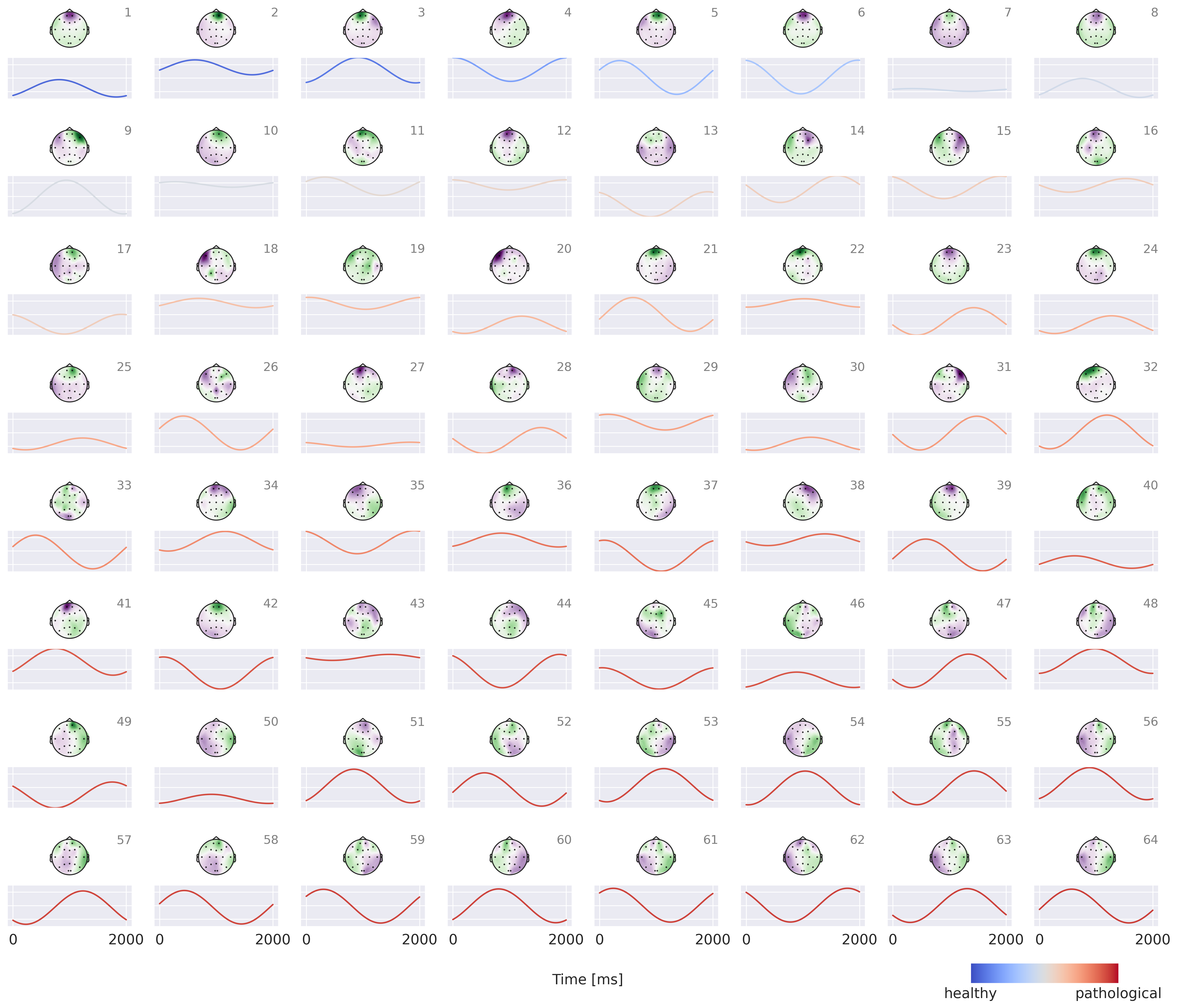
Fig. 52 Spatiotemporal patterns for EEG-CosNet trained on lowpassed data below 0.5 Hz. Note large frontal components associated with healthy class.

Visualization of the EEG-CosNet in Fig. 52 contain strong frontally components associated with the healthy class and components in temporal areas associated with the pathological class. The temporal components are in line with the per-electrode visualization, and the frontal components were already visible as differences in mean signal values in the class prototypes on the original data.

Fourier-GMM Visualizations

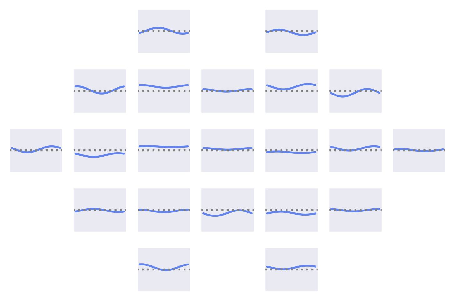
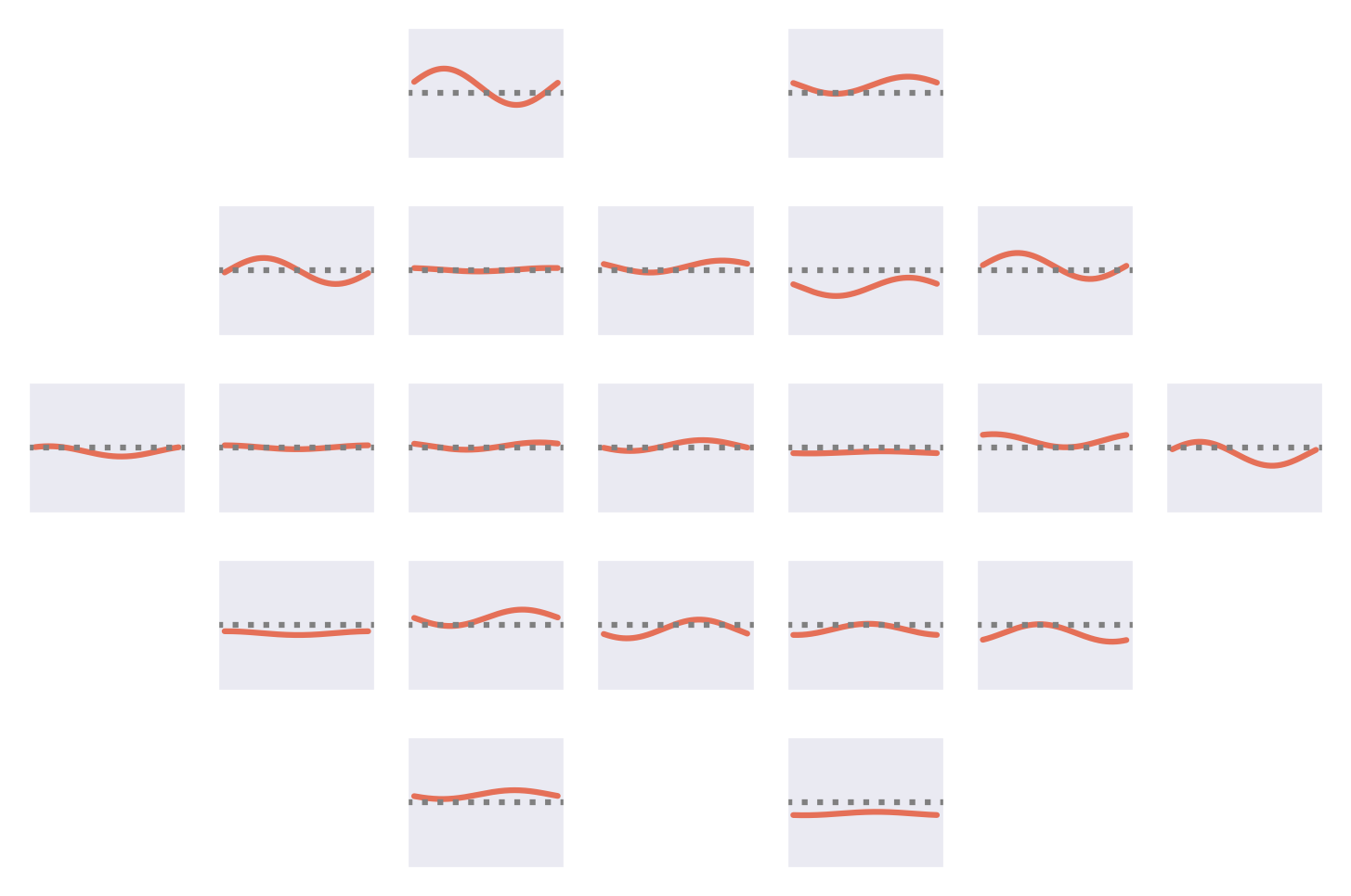
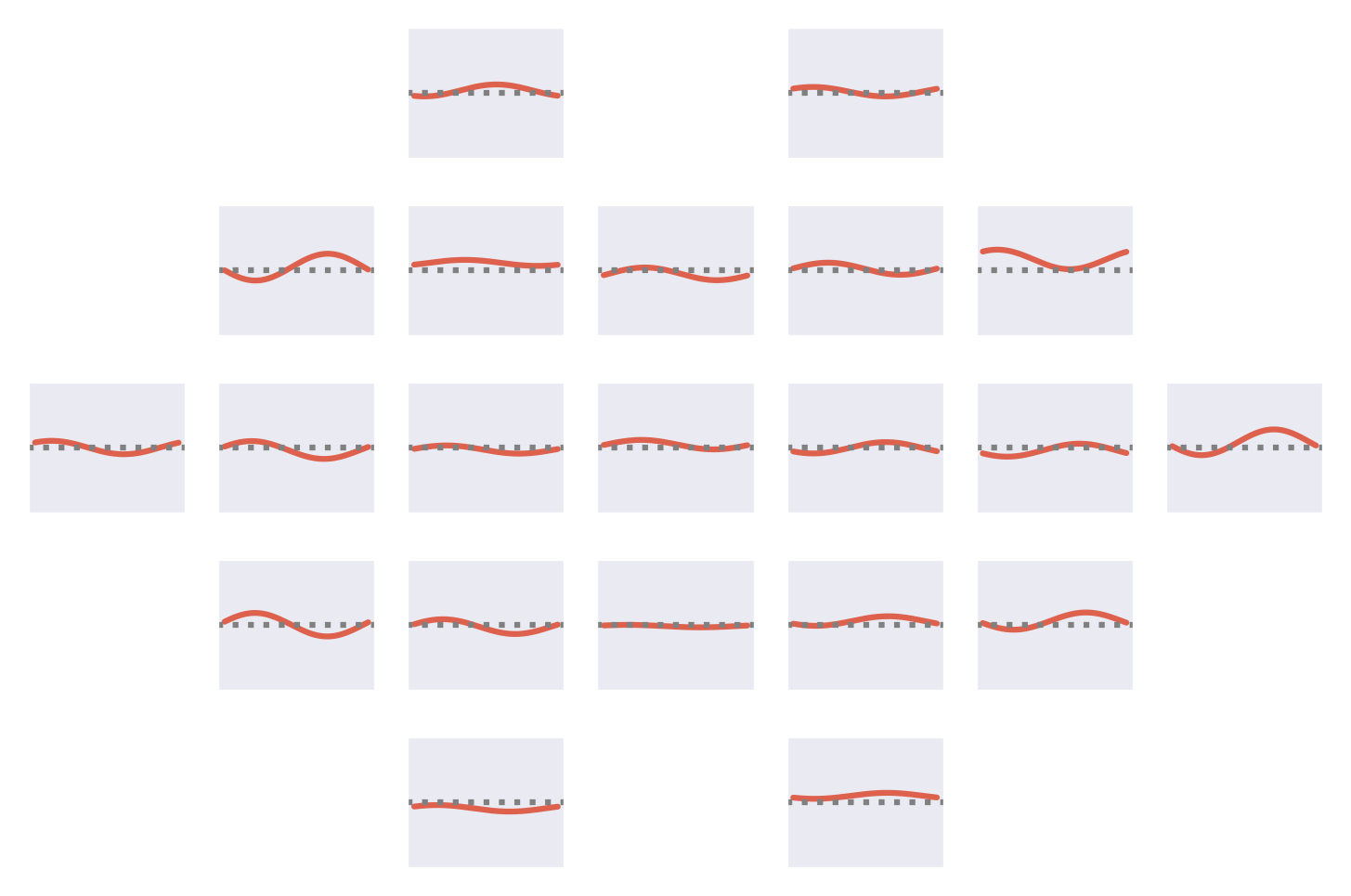
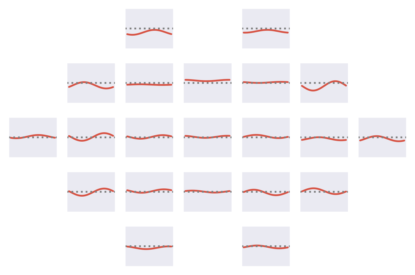
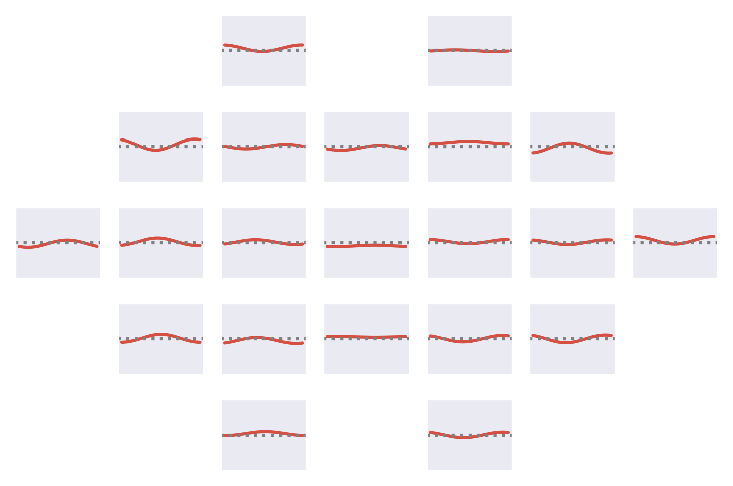
Fig. 53 Means of the Fourier-GMM mixture components shown after inversion into input space. Note clearly visible frontal signals in the components for the healthy class.

Fig. 54 Means of the Fourier-GMM mixture components in Fourier space. Scalp plots for 0-Hz bin, real and imaginary values of 0.5-Hz bin. Components sorted by pathological class weight, also shown as colored text in top right of each component. Colormaps scaled per frequency bin. Note strong frontal components for mixture components associated with healthy class.

Visualizations of the Fourier-GMM in Fig. 54 again show frontal components associated with the healthy class and other components, with spatial topographies that include temporal areas, associated with the pathological class.

Overall, the visualizations consistently indicate a frontal component predictive for the healthy class and other components, with a spatial topography that often includes temporal and nearby areas, predictive for the pathological class.

Open Questions

• What other methods may in the future help understand discriminative features in the EEG signal?